Arbitrary Lagrangian Eulerian form of flowfield dependent variation (ALE FDV) method for moving boundary problems

(1)

ARBITRARY LAGRANGIAN-EULERIAN FORM OF

FLOWFIELD DEPENDENT VARIATION (ALE-FDV)

METHOD FOR MOVING BOUNDARY PROBLEMS

BY

MOHD FADHLI BIN ZULKAFLI

A thesis submitted in fulfilment of the requirement for the

degree of Doctor of Philosophy

Kulliyyah of Engineering

International Islamic University Malaysia

(2)

ABSTRACT

(3)

LIST OF TABLES

Table No. Page No.

4.1 CPU time per time step for each number of cells 72

4.2 Velocities maximum error norm, L∞(ui) 80

4.3 Summary of unstructured mesh 90

4.4 Velocities maximum error norm for three-dimensional wavy mesh

98

4.5 Comparison of CPU time taken by ALE-FDV and ANSYS Fluent

(6)

[image:6.595.105.510.156.781.2]

LIST OF FIGURES

Figure No. Page No.

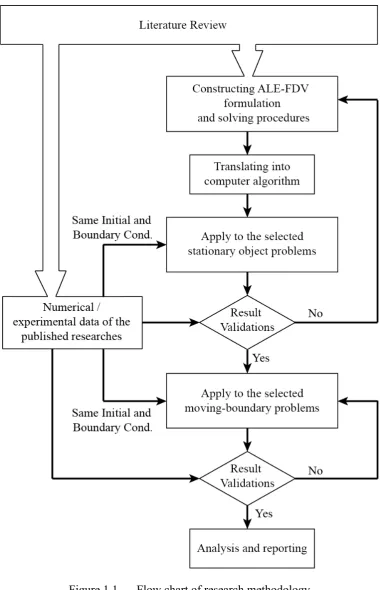
1.1 Flow chart of research methodology 7

3.1 Definition of cell I in one-dimensional space 36

3.2 Definition of cell I for vertex-centered finite volume 39

3.3 Definition of cell I for cell-centered finite volume 42

3.4 Flowchart of ALE-FDV method’s main program 49

3.5 Flowchart of ALE-FDV method’s sub-program 50

3.6 Flowchart of Block Tri-diagonal algorithm 51

3.7 Flowchart of Restart GMRES algorithm 52

4.1 Distribution of modulus z for several Courant numbers and its

relation to the FDV parameter s1 58

4.2 Distribution of modulus z for several values of FDV parameter

s1

59

4.3 Distribution of modulus z for several _η when v = 1.0 and s1 = 0.25

59

4.4 Comparison of exact and numerical solution of Sod shock tube at time instant, t = 6.1 msec

62

4.5 Comparison of density profile at the location of contact discontinuity for different cells number 62

4.6 FDV parameters and Mach number profile at time instant, t =

6.1 msec 63

4.7 Numerical results for interaction of two-blast shockwave problem at time instant, t = 0.038 65

4.8 Numerical results for solution of half-Riemann problem at time instant, t = 0.2

(7)

4.10 Entropy errors 71

4.11 Pressure profile at several time instants 73

4.12 FDV parameters and local Mach number at several time

instants 74

4.13 Position of the wall 75

4.14 Pressure profile at several time instants 77

4.15 Motion of the deformable mesh 80

4.16 Density contour at time t = 0.1 83

4.17 Comparison between exact solutions and numerical solutions of pressure coefficient along x2 = 0 at t = 0.1

83

4.18 Comparison of density error between deformed and stationary mesh

84

4.19 Pressure contour at several angles of attack (left figures: present, right figures: Murman et al., 2003)

86

4.20 Comparison of lift coefficient 86

4.21 Comparison of lift and drag coefficient 88

4.22 Comparison of vorticity profile at AoA = 44 degrees 89

4.23 ω = 1.0 (left figures: present, right figures: Sen et al., 2013) 91

4.24 _ω = 3.0 (left figures: present, right figures: Sen et al., 2013) 92

4.25 Experimental results by Badr et al. (1990) 93

4.26 Flow field at t = 8.0 for case ω = 1.0 94

4.27 Average lift and drag coefficient of each mesh for case ω = 1.0 95

4.28 The wavy mesh for the three-dimensional free stream preservation test

98

4.29 Mach number and parameter s1 profile at different time instants and angle of attacks

100

4.30 Comparison of computed lift and moment coefficient with experimental and numerical data

(8)

4.31 Streamline profile of present method (left) and Kim (2009) (right) at different rotation speed

104

4.32 Comparison of flight path 107

4.33 Streamline pattern of anti-clockwise spinning sphere at its initial position

108

(9)

LIST OF SYMBOLS

Roman symbols

a Convection Jacobian

b Diffusion Jacobian

c Diffusion gradient Jacobian

E Total energy per unit mass

F Inviscid flux

G Viscous flux

I Vertex/ cell element index number

J Neighbour vertex/ cell element index number

M Mach number

n Normal vector

p Pressure

Pr Prandtl number

Re Reynolds number

sa First-order implicitness parameter

sb Second-order implicitness parameter

s1 First-order convection FDV parameter

s2 Second-order convection FDV parameter

s3 First-order diffusion FDV parameter

s4 Second-order diffusion FDV parameter

t Time

(10)

U Conservative variables

vm Mesh velocity

xi Cartesian coordinates

Greek symbols

Δ Changes in time/ space

δij Kronecker delta

ε Internal energy per unit mass

Γ Control surface/ cell boundary

γ Specific heat ratio (Ideal gas = 1.4)

µ Dynamic viscosity coefficient

ρ Density

τij Viscous stress tensor

Ω Control volume/ cell volume

Subscripts

I Cell indices

I(J) Neighbour cell of cell I

i, j, k Spatial direction indices

IC Interior cell

m mesh

n Normal direction

T Total value

(11)

w Wall surface

∞ Free stream condition

Superscript

m GMRES iteration

(12)

LIST OF ABBREVIATIONS

ALE Arbitrary Lagrangian-Eulerian

ALE-FDV Arbitrary Lagrangian-Eulerian form of Flowfield Dependent Variation AoA Angle of Attack

CFD Computational Fluid Dynamics CFL Courant-Friedrichs-Lewy CBS Character-based Split

DGCL Discrete Geometric Conservation Law

DGFEM Discontinuous Galerkin Finite Element Method et al. (et alia): and others

FDV Flowfield Dependent Variation FDM Finite Difference Method FEM Finite Element Method FVM Finite Volume Method GCL Geometric Conservation Law GMRES General Minimal Residual

GRAFSS General Relativistic Astrophysical Flow And Shock Solver HOC Higher-Order Compact

HOC-FDV Higher-Order Compact Flowfield-Dependent Variation IB Immersed Boundary

i.e. (id est): that is

LSGR Least Square Gradient Reconstruction MFDV Modified Flowfield Dependent Variation

MUSCL Monotone Upwind Schemes for Conservation Law PDE Partial Differential Equation

PISO Pressure Implicit with Splitting of Operators

(13)

CHAPTER ONE

INTRODUCTION

1.1 INTRODUCTION

Governing equations in fluid mechanics are a coupled system of nonlinear partial

differential equations, which are difficult to solve analytically and to date except for

some particular problems, there is no general closed-form solution to these equations.

Thus, numerical approach is important in order to study and analyze the problems

involving fluids. In fluid mechanics, the area that studies such an approach is

Computational Fluid Dynamics (CFD), and its development began with the advent of

the computer in the 1950s. CFD is important as a research and design tool today

because the development of modern technologies such as high-speed transportation,

electronics and biotechnologies also rely on the understanding of fluid mechanics.

Major basic techniques used in the solution of partial differential equations in

general and CFD in particular are Finite Difference Methods (FDM), Finite Element

Method (FEM) and Finite Volume Method (FVM). FDM is easy to formulate but

because a structured mesh is required, it has difficulties with multi-dimensional

problems that involve complex geometries. In contrast, complex geometries and

unstructured meshes are easily accommodated by FEM but it uses large computer

memory, thus slow for large problems and not well suited for turbulent flows.

FVM however, has an advantage in memory usage and speed for very large

problems. This method is based on the discretization of the integral form of nonlinear

partial differential equations (PDE) into finite control volumes and control surfaces. It

(14)

applicable to unstructured grids and complex geometries. Furthermore, the system of

algebraic equations by finite volume methods enforces the conservation of all

variables across the control surfaces. Therefore, the conservation of mass, momentum

and energy are assured in the formulation itself while variables may not be

continuously differentiable across shock or other discontinuities, which is an

advantage for high-speed flow problems.

In CFD, the problems are usually solved by different techniques depending on

the physical properties of the flows. For example, incompressible flows are analyzed

using the pressure-based formulation but compressible flows are analyzed using the

density-based formulation. In dealing with the domains, which contains flows of all

speed with various physical properties, where the equations of state for compressible

and incompressible flows are different, and where the transitions between laminar and

turbulent are involved, very special and powerful numerical treatments are needed.

The so-called Flowfield Dependent Variation (FDV) theory, which was first

introduced by Chung (1999), has been devised toward resolving these issues. The

theory introduced the so-called FDV parameters, which are dependent on the gradient

of changes between flow variables (e.g. Mach number or Reynolds numbers) of local

adjacent nodal points in the computational domain. Because of these parameters, the

terms containing the fluctuation variables in the FDV equation automatically follow

the current physical phenomena and adequate numerical controls (artificial viscosity)

are automatically activated according to the current flow field physics. The numerical

scheme of the FDV equation itself will then adjust accordingly for every node based

(15)

For the numerical simulation and analysis of objects that move within the flow,

the objects usually are made static relative to the flow in the computational domain,

similar to the wind tunnel experiment. However, there are many situations when the

objects are needed to move or deform in the computational domain such as airfoil

oscillations, wing flutter, and rotating propellers problems. This is one of the

important issues in CFD applications, because the simulations of the flow around

moving objects require special interpolation methods to handle the moving

boundaries. Methods for moving computational mesh have been studied actively by

the CFD community because of their engineering importance. One of the most

popular techniques in solving moving boundaries problems is Arbitrary

Lagrangian-Eulerian (ALE), which combines Lagrangian and Lagrangian-Eulerian description of a continuum,

i.e. fluid and solid, in one numerical scheme.

The present research studies the combination of FDV method and ALE method

in finite volume form. The finite volume form would make this method applicable to

complicated geometries of moving bodies and by combining FDV with ALE method,

it would give an accurate prediction of the interactions between fluid and the moving

bodies. Therefore, it is expected that the proposed method will provide a new

technique of resolving accurately the interaction of arbitrary bodies in arbitrary flow

fields.

1.2 PROBLEM STATEMENT

Unified Computational Fluid Dynamics (CFD) method has been the aim of the CFD

community in recent years. The need for a unified method arises because in CFD,

different type of flow problems need different type of method to solve, but in reality

(16)

may coexists with high speed flow area such as in the cases of aircraft landing or

take-off configurations where the free stream Mach number is much less than the local

Mach number around the high-lift devices of the aircraft. Flowfield Dependent

Variation (FDV) method has been introduced to resolve these problems, however this

method is currently limited to stationary bodies and has not yet been used to handle

moving boundary problems. This research proposes to combine FDV method with

moving boundary interpolation technique, ALE method for solving moving boundary

problems because in some cases, deformation and motion of the bodies need to be

taken into account in order to get accurate results without ignoring its physical

properties as well as the existence of many different flow regimes within a flow field.

1.3 RESEARCH PHILOSOPHY

The philosophy of this research is to combine the advantages of FDV theory with a

moving body technique, the ALE method, in order to develop a robust and versatile

method, which could be used for the computation of flow fields with moving

boundaries. The philosophy is driven by the need to consider the deformation and/or

movement of bodies in a flow in which to date, the FDV theory has not been applied.

The philosophy is based on obtaining the parameters of the FDV equations from the

current flow field variables at each time step and every grid point which are used to

adjust governing equations in each flow region according to the current flow field

situation. The combination of ALE and FDV method will be used to handle the

problems involving moving boundaries in a flow. Meanwhile, the finite volume

method gives the ALE-FDV formulation, the capability to solve flow problems

(17)

1.4 RESEARCH OBJECTIVES

The objectives of this research are as follows.

• To develop a technique which could be used for wide ranges of

compressible-incompressible, viscous-inviscid, laminar-turbulent, and

high-low speed flows for moving boundary problems.

• To combine FDV method and a moving body interpolation technique,

named ALE method for solving flow problems involving moving

boundaries.

• To apply the proposed method to solve three-dimensional inviscid and

viscous flow problems involving moving boundaries by developing an

algorithm and translate it into an efficient computer code.

• To investigate such combinations that will satisfy the stability requirement

as well as guarantee accuracy and efficiency.

1.5 RESEARCH METHODOLOGY

The methodology of this research will focus on the development of the proposed

method based on numerical work. The numerical work will be carried out using

traditional way of CFD, starting with pre-processing, then solving process, and ending

with post-processing. Pre- and post-processing will be performed using commercial

softwares, Gambit as mesh generation software and Paraview as visualization

software. The solving process will be carried out using FORTRAN code on a UNIX

based machine. The steps of algorithm development for the proposed method will be

done as follows:

a) The step begins by expanding conservative variables (i.e. density,

(18)

series. This expansion is done with the addition of implicitness parameters

into the first and second time derivatives of that series. Next, the time

derivatives are changed into spatial derivatives by substituting the

Navier-Stokes equations in that series to construct the FDV formulation.

b) The general formulation of ALE-FDV method is derived by combining

ALE technique with the FDV formulation. The formulation is then

discretized using appropriate finite volume method.

c) Strategies to solve the ALE-FDV formulation are then constructed and

translated into computing algorithm. This algorithm is then written in

FORTRAN language as the solver code.

d) Then, selected stationary body in one-dimensional problems flow is

solved using the developed solver and numerical as well as experimental

data available in the literature is used to validate the solver.

e) If the solutions of the stationary body problems are valid, several

one-dimensional moving boundary problems are selected and solved using the

complete solver for the validation and analysis process.

f) Finally, ALE-FDV method is applied to two and three-dimensional flow

problems by repeating steps b to e.

To summarize, the following flow chart shows the overall methodology of this

(19)

[image:19.595.126.509.66.657.2]

(20)

1.6 SCOPE OF RESEARCH

This study focuses on developing a new numerical scheme that combines the FDV

method and ALE method. The proposed method is spatially discretized using

appropriate finite volume method. A flow solver, called as ALE-FDV solver is

developed by translating the discrete formulation into an algorithm. In order to

validate the scheme, the developed solver is applied to several benchmark one, two

and three-dimensional flow problems. The flow problems involving moving mesh and

fluid-structure interaction in inviscid or viscous fluid are also in the scope of this

work.

1.7 THESIS ORGANIZATION

This thesis is organized by dividing it into five chapters. This chapter, which is the

first chapter, gives an introduction and background of FDV and ALE method as well

as demonstrates the importance of extending FDV method into the application of

moving boundaries and fluid-structure interaction problems. Problem statements,

research philosophy, objectives, methodology and scope of the research are also

explained in the first chapter. Second chapter presents a review of previous studies

and works that are relevant to this research. The review covers past and recent works

related to the FDV and ALE methods as well as other works involving moving

boundaries and fluid-structure interaction applications.

The third chapter explains the derivation of the ALE-FDV method and the

technique to discretize it with finite volume method. The strategies to apply

ALE-FDV method and the algorithm used in this research are also explained in detail in the

(21)

numerical results and verification of ALE-FDV method by comparing with previous

relevant works are discussed in the same chapter. Finally, the fifth chapter concludes

this research works and findings, highlights the main contributions of the research and

(22)

CHAPTER TWO

LITERATURE REVIEW

2.1 INTRODUCTION

Interaction between a solid and a fluid is a common phenomenon either in nature or

induced by human activities. Such interactions happen in various disciplines and at

different scales, which can be modeled through experiments or simulated using

computational method. In a modern world, computer simulation has become an

important tool because it provides an economical approach as well as additional

insight to the analysis of such fluid interactions.

The numerical approach in fluid mechanics, Computational Fluid Dynamic

(CFD), has been developed in the 1950s and since then has been extended by

researchers in order to allow investigation on various complex fluid interactions. CFD

is being used extensively in many industrial sectors and is advancing rapidly as more

complex fluid interaction become available and simulation on larger scale is more in

demand today.

As the flow simulation become larger and complex, development of more

accurate and efficient numerical scheme has become significant. One of the numerical

approaches called Flowfield Dependent Variation (FDV) method has been developed

towards resolving complex flow interaction problems. In this chapter, a review on the

development and application of FDV method and other similar method will be

presented. At the same time, many fluid and solid interaction problems require

(23)

presents an overview on the development and application of such grid interpolation

techniques. This chapter will be ended by a summary of all reviews and conclusion on

the advantages and drawbacks of numerical schemes used in the reviewed literatures.

2.2 UNIFIED CFD METHOD

Compressible flow field solvers use density as their primary unknown variable while

artificial compressibility method (Chorin, 1967) and pressure correction method

(Harlow and Welch, 1965) are the two approaches that have been widely used as

incompressible flow solvers. The problem with compressible flow solver is that some

areas of the flow would be incompressible, thus make it unsuitable for the

compressible flow solver alone to compute the entire flow field. Since the solution of

incompressible flow can be obtained as part of the compressible flow formulation, the

method of extending the function of compressible flow solver has been actively

studied (Wesseling, 2000).

Either explicit or implicit time stepping scheme can be used to solve the

governing equations numerically. However, an explicit scheme needs to satisfy the

stability condition in order to produce solutions of the problems. In particular, the

stability condition, known as Courant-Friedrich-Lewy (CFL) condition dictates the

Courant number (i.e., ratio of physical propagation speed to numerical propagation

speed) must be less than unity (Courant, Friedrichs and Lewy, 1967). In other words,

the time needed for the numerical information to propagate in a spatial distance ∆x

must be smaller than the time of physical information propagation in that same

distance. Moreover, the time needed for the numerical information to propagate will

become much smaller if acoustic effects are present in low-subsonic flow. When this

(24)

many small steps to be solved. Moreover, often-wrong results are obtained when a

stiff system of equations are solved by carrying out very large number of small time

steps as reported by Turkel, Fiterman and Van Leer (1993) and Guillard and Viozat

(1999).

In order to resolve the problem, some numerical schemes such as

preconditioning techniques are developed. This scheme alleviates the problem by

modifying the governing equations artificially by multiplication of the time-derivative

with a specific preconditioning matrix. While the scheme resolved stiffness and

accuracy problem for stationary solutions, the time accuracy is lost due to the

modification of time derivatives in the governing equations. Therefore, to compute

unsteady flows, the preconditioning method has been combined with dual time

stepping method in order to restore the accuracy in time (Weiss and Smith, 1995). It

has been shown that dual time stepping is more efficient than physical time stepping

used by the original compressible flow solver. However, because of the large number

of pseudo-time steps required for each physical time step, the efficiency lags behind

incompressible flow solvers (Wesseling, 2000). As remarked by Paillére, Clerc,

Viozat, Toumi, and Magnaud (1998), implicit time stepping scheme must be used if

the explicit time stepping scheme requires a very small time step to satisfy the

stability condition.

A different approach has been taken by Yoon and Chung (1996), where they

introduced the so-called mixed explicit implicit generalized Galerkin spectral element

method (MEI-GG-SEM). Unlike traditional methods, the so-called flow field

dependent parameters detect the physical properties of the fluid and then

(25)

flow where mesh refinement were carried out adaptively until shock waves were

resolved in which the traditional turbulence model is no longer needed.

Complexities of fluid phenomena are not only due to the co-existence of

compressible and incompressible flow, it also includes transition to turbulence,

relaminarization, flow separation and transition between viscous and inviscid flow

regions. Instead of focusing only on the incompressible and compressible flow

mixture problems, a new approach called the flow field dependent mixed

explicit-implicit (FDMEI) method has been developed in attempt to resolve the complexities

of fluid phenomena in all speed flow regimes (Chung, 1997a, 1997b; Yoon, Moon,

Garcia, Heard, and Chung, 1998). Based on the flowfield dependent variation (FDV)

theory, this method uses FDV parameters which depend on the change of either Mach

numbers, Reynolds numbers, Peclet numbers, or Damkohler numbers at adjacent

nodal points to detect physical properties of each nodal points. Peclet number or

Damkohler number is used for high speed compressible flow problems such as in

hypersonic flow or chemically reactive flow problems such as in combustion. Peclet

number is defined as the ratio of convective to diffusive strength (Wesseling, 2000)

while Damkohler number defined the relationship between chemical reaction and

flowfield transport phenomena such as convection, diffusion or heat conduction

(Chung, 2002).

Appropriate numerical schemes are provided to each nodal point if necessary

by calculating and updating the values of these parameters at each time step. Yoon et

al. (1998) used FDMEI method to compute flow over a flat plate, supersonic flow on a

compression corner, three-dimensional duct flow, and lid-driven cavity flow. Their

results showed good agreement with experimental and other published numerical

(26)

resolve mutual interactions and transition between viscous/ inviscid, compressible/

incompressible, and laminar/ turbulent flows.

2.3 FLOWFIELD DEPENDENT VARIATION (FDV) METHOD

The original idea of FDV theory began from the need to address the physics involved

in shock wave turbulent boundary layer interactions (Chung, 1999). In this situation,

transition and interactions of inviscid/ viscous, compressible/ incompressible, and

laminar/ turbulent flows constitute not only the physical complexities but also

computational difficulties. This is where the very low velocity in the vicinity of the

wall and very high velocity far away from the wall co-exist within the domain of

study. Implicitness parameters were initially introduced in the expansion of

conservative variables in the Taylor series up to the second order time derivatives.

The series are then used in the Navier-Stokes system of equations so that these

parameters could be used in solving the flow field interaction. These parameters are

characterized into two categories, namely first and second order convection/diffusion

parameter. In particular, the first order parameters ensure the solution accuracy and

second order parameters assist in the solution stability, and both serve as physical

parameters to allow the transitions and interactions of different types of flow to be

automatically accommodated.

Moreover, flowfield-dependent variation formulations have been addressed by

Schunk, Canabal, Heard, and Chung (1999) as a strategy toward unification of finite

difference, finite element, and finite volume methods. All the physical phenomena are

taken into account in FDV equations, so that spatial discretization will not dictate the

(27)

introduced in FDV equations play significant roles as adjusting the governing

equations (hyperbolic, parabolic, and/or elliptic), resolving various physical

phenomena, and controlling the accuracy and stability of the numerical solution. The

theory is verified by a number of example problems addressing the physical

implications of the variation parameters, which resemble the flow field itself. Using

finite difference method as spatial discretization of FDV equations, Schunk et al.

(1999) showed numerical results of three-dimensional triple shock/boundary layer

interaction matched with experimental results and finite difference calculation using

k-ε model as reported by Garrison, Settles, and Hortsman (1996), thus indicated that

FDV theory was robust enough to adequately model complex flow phenomena.

FDV theory also has been applied in high-energy astrophysics problems,

particularly to those containing shock waves and high-speed flow. Richardson, Chung,

Karr, and Pendleton (2000) proposed the FDV theory as a method to accurately solve

very high-speed flow problems and capturing relativistic shocks. Instead of Mach

number, Lorentz factor, which describe the velocity of an object relative to the speed

of light (Corcoran, 2010), is used to dictate the FDV convection parameters. The

theory has been applied in relativistic hydrodynamic equations to solve relativistic

shock tube problems. Furthermore, they also presented FDV method for solving

general relativistic non-ideal hydrodynamics (Richardson and Chung, 2002a).

Non-ideal flows are where radiation, magnetic forces, viscosities, and turbulence play an

important role. Relativistic effects become pronounced in such cases as jet formation

from black hole magnetized accretion disks, which may lead to the study of

gamma-ray bursts. Richardson and Chung (2002b) implemented the FDV theory to obtain

general relativistic astrophysical flow and shock solver (GRAFSS) which is a

(28)

geometries. Richardson, Cassibry, Chung, and Wu (2010) have demonstrated the

capability of the finite element form of FDV method in physical applications that have

widely varying spatial and temporal scales. The use of a finite element formulation

also adds capabilities such as flexible grid geometries and exact enforcement of

Neumann boundary conditions. The author presented the results of

converging/diverging nozzle, which contains both incompressible and compressible

flow in the flow field over a range of subsonic and supersonic regions. The results

showed that the finite element formulation is stable and accurate for a range of both

Mach numbers and Lorentz factors while its accuracy are comparable to other

methods and slightly better than Total Variation Diminishing (TVD) method.

Heard (2007) utilized the FDV parameters for adaptive mesh refinements. FDV

equations were solved using an element-by-element GMRES solver with the elements

grouped together to allow the element operations to be performed in parallel. Besides

dictating the physical properties of the flow field, FDV parameters are used as error

indicators for a solution-adaptive mesh. The finite element grid is refined as dictated

by the magnitude of FDV parameters. This method is comparable to those where the

grid is refined using primitive variable error indicators, and requires less

computational time to generate the grids. The use of parallel processing in performing

some element operations is shown to reduce the wall clock time by approximately 40

percent in going from one to eight processors. The algorithm's ability to solve a flow

field containing various kinds of interactions is demonstrated by solving a variety of

fluid flow conditions ranging from low-speed incompressible flow to compressible

flow containing shock waves, and the refinement of finite element grid to further

(29)

FDV parameters were modified by Megahed, El-Mallah, and Girgise (2006) to

improve the understanding of physical meaning of the variation parameters. The

modified method, MFDV method was applied to the Euler equation with standard

Galerkin finite element method as its spatial discretization. Two well-known cases of

supersonic internal flow; shock reflection problem and compression corner problem

were solved and the results were shown to have a good agreement with other

published literature. Furthermore, three other cases of supersonic internal flow; half

wedge in supersonic wind tunnel, extended compression corner problem, and circular

arc problem also has been solved. All of the numerical solutions are comparable with

analytical and numerical solutions obtained by other established methods, thus

showed the ability of the MFDV method to solve problems involving supersonic

internal flow.

FDV theory also has been combined with higher-order compact method (Hirsh,

1975; Lele, 1992; Mawlood, Basri, Asrar, Omar, Mokhtar, and Ahmad, 2006; Elfaghi,

Asrar, and Omar, 2010) which is generally a technique that use fewer number of nodal

points to obtained high order finite difference approximation as opposed to classical

finite difference method. Originally developed by Elfaghi et al. (2010), Higher-Order

Compact Flowfield-Dependent Variation (HOC-FDV) method used implicit fourth

order compact differencing Hermitian (Pade-type) scheme to approximate the spatial

derivatives in FDV equations. HOC-FDV method has been applied to solve up to

two-dimensional problems such as Sod-shock tube problem, interaction of two-blast shock

waves, and flow past NACA0012 airfoil (Elfaghi, Asrar, and Omar, 2009a). The same

method also has been used in solving full Navier-Stokes equations such as nonlinear

viscous Burgers equation and transient Couette flow (Elfaghi, Asrar, and Omar,

(30)

operate in various flow regimes without using any special treatments due to the

capability of the FDV method. Moreover, HOC-FDV is more efficient than FDV

method as well as other conventional high-order methods because less stencil points is

required to obtain solutions with the same accuracy.

2.4 FLOWS WITH MOVING BOUNDARIES

Moving boundary problems in CFD applications are the cases where boundaries of the

bodies (or obstacles) in a flow are moving and/or deforming. For example, airfoil

oscillations, wing flutter, accelerated/decelerated aircraft, rotating propellers, fast

turning cars, reciprocating engines, suspension bridges vibration, flapping wings,

pulsating blood vessels, etc. Some movements of these boundaries are relatively small

but when they undergo large displacements, rotations or deformations, the effects of

fluid-body (or fluid-structure) could not be ignored. The need to solve such kind of

flow problems using dynamic mesh (i.e. the moveable/deformable body-conformal

grids system) has attracted many researches to develop various kinds of moving grid

interpolation techniques. One of the body-conformal moving grid interpolation

technique that is widely used in fluid and solid mechanics is Arbitrary

Lagrangian-Eulerian (ALE) method. However, simulation of largely deformable objects using

dynamic mesh is quite unstable and requires costly grid generation methods.

Therefore, such simulations are widely performed using stationary mesh

(non-conformal grid system) with the so-called Immersed Boundary (IB) method (Peskin,

(31)

2.4.1 Arbitrary Lagrangian-Eulerian (ALE) Method

Numerical algorithms using ALE method combine two classical kinematic

descriptions of continuum (i.e. fluid and solid) mechanics; Lagrangian and Eulerian

description. Lagrangian algorithms, in which each nodal point in the computational

domain follow the movement of associated structures, are mainly used in solid

mechanics. In contrast, Eulerian algorithms allow the continuum to move with respect

to the fixed computational grids, thus widely used in fluid mechanics. By combining

both algorithms, the computational grid can follow the moving objects in a

Lagrangian way, while the fluid is still seen in an Eulerian manner (Donea, Huerta,

Ponthot, and Rodríguez-Ferran, 2004).

ALE method was originally introduced in finite difference formulation (Hirt,

Amsden, and Cook, 1974), and has been successfully implemented in finite volume

and finite element formulations.Guardone, Isola, and Quaranta (2011) discretized the

ALE formulation of Euler equations with finite volume method. They adopted

edge-swap technique to improve the quality of triangular or tetrahedral cells in the

deformation mesh and thus allow the boundaries to encounter large displacement. The

technique is applied on translating and oscillating NACA 0012 airfoil case in which

the mesh undergo large deformation.

Habchi, Russeil, Bougeard, Harion, Lemenand, Ghanem, Valle, and

Peerhossaini (2013) developed a fluid-structure interaction solver using finite volume

approach. Both governing fluid flow equation and structural displacement equation

are discretized using finite volume method. ALE formulation is used to handle

displacement of fluid-structure interfaces in the deforming mesh. Some benchmark

two-dimensional problems such as lid-driven cavity with flexible bottom edge, elastic

(32)

problem have been used to validate the solver. Through the combination of Pressure

Implicit with Splitting of Operators (PISO) algorithm and Semi-implicit Method for

Pressure-Linked Equations (SIMPLE) algorithm to solve fluid governing equation,

they obtained accurate solutions by using large time steps.

Feistauer, Kučera, and Prokopová (2010) discretized the ALE form of

compressible Euler equations using discontinuous Galerkin finite element method

(DGFEM). Semi-implicit time discretization is used to avoid CFL-stability constraint

thus allowing large time step to be taken for low Mach number problem. Then,

Feistauer, Hasnedlová-Prokopová, Horáček, Kosík, and Kučera (2013) extended the

method for viscous flow problems. They employed DGFEM as the discretization

technique on ALE form of compressible Navier-Stokes equations. They showed that

based on the validation of several numerical tests, the method can be applied to the

fluid flow problem involving elastic structures.

Sun, Zhang, and Ren (2012) improved the characteristic-based split (CBS)

scheme in ALE framework by reformulating the previous ALE-CBS scheme.

Standard Galerkin finite element method is used for spatial discretization of governing

flow equation while spring analogy method proposed by Blom (2000) is used in the

moving mesh strategies. The improved ALE-CBS scheme is applied to the broken

dam problem and the flow around oscillating circular cylinder. They found that the

improved ALE-CBS scheme demonstrates better accuracy even using coarse mesh

with large time step and is unaffected by mesh velocities in contrast to the former

existing ALE-CBS scheme.

Implementation of ALE method requires re-meshing formulation to update the

(33)

in the stability and accuracy of ALE method, many researches have enforced

Geometric Conservation Law (GCL) when using this method.

The concept of GCL was derived by Thomas and Lombard (1979) in order to

resolve the difficulties with maintaining global and local volume conservation due to

the boundary-conforming coordinate transformation applied on flow computation

involving moving boundaries. During such computation, the magnitude of

transformation Jacobian (used to map variables in Cartesian coordinate system to a

boundary-conforming curvilinear coordinate system) changes as the geometries of the

boundary change in time. They found that, unsatisfying conservation of local volume

due to such changes leads to erroneous solution. Therefore, GCL was addressed as a

way to govern the changes so that it will not violate the local volume conservation.

The concept was further investigated by (Guillard and Farhat, 2000) for solving

time-dependent governing equations on dynamic mesh. They then introduced Discrete GCL

(DGCL) as a useful guideline to evaluate geometric quantities involving grid positions

and velocities. The law states the evaluation of such quantities should be conducted in

a way that the numerical scheme used for integrating the flow equations must preserve

a uniform flow field, independently of the mesh movement.

Since then, many researchers have studied the impact of GCL on solution

accuracy. Thomas and Lombard (1979) implemented the GCL for density-based finite

difference schemes on structured grids while Shyy, Udaykumar, Rao, and Smith

(1996) implemented the GCL for pressure-based finite volume schemes. Lesoinne and

Farhat (1996) developed first order time accurate scheme preserving the GCL using

density-based ALE finite volume and finite element schemes on unstructured grids

(34)

ALE finite volume schemes. Most studies show that not satisfying the GCL leads to

wrong solutions or spurious oscillations in the solutions.

Mihara, Matsuno, and Satofuka (1999) presented an iterative finite-volume

approach for unsteady coupled system of fluid and body motion in compressible

flows. Similar to the dual-time or pseudo-time concept, inner iteration was carried out

at every time step in order to satisfy the geometric conservation laws and to ensure

accuracy. Gun-tunnel simulation was carried out using the method and based on the

results, the method always satisfies the conservation laws independent of the CFL

condition. The approach was further improved by using solution-adaptive

moving-grid method (Sato, Matsuno, Nakagawa, and Satofuka, 2001). The improved version

was validated by comparing numerical solutions of cylindrical implosion problem. It

was proven to be more accurate than the solutions of uniform grid. On the other hand,

Yamakawa and Matsuno (2004) presented the iterative finite volume method that

includes algorithm for eliminating and merging cells of unstructured moving grids.

The new method was developed for compressible flows and it was applied to a gun

tunnel problem and two bodies docking and separating in a supersonic flow problem.

Visbal and Gordnier (2000) extended the HOC schemes for the solution of

Navier-Stokes equations on moving grids. The authors used up to sixth order accurate

Pade-type compact finite difference scheme combined with low-pass filtering

technique while carried out time-marching using explicit (fourth order Runge-Kutta)

and implicit (Newton-like sub iterative Beam-Warming scheme) time-integration

method. Transformation Jacobian is evaluated at each time step using GCL in order to

ensure free stream preservation. The extended scheme is applied on two and

(35)

pitching NACA 0012 airfoil and the simulation of aeroelastic interaction arising from

viscous flow past over a flexible panel. The simulation of pitching NACA 0012 airfoil

was carried out using rotating (the grid rotates as the airfoil pitched at some angle)

grid and deforming (the grids near airfoil boundaries distorted as the airfoil pitched at

some angle) grid. Good agreement of both results indicated the robustness and

versatility of this method. Furthermore, the resulting pressure field due to interaction

of boundary layer and flexible panel exhibit acoustic radiation while the same

phenomena does not arise in non-interacting case, thus showing the importance of

computing fluid-structure interaction to capture the real physics behind such

phenomena.

Kamakoti and Shyy (2003) state that GCL have been proven to be a key

component of Computational Aeroelasticity problems specifically involving

deforming grids. They developed a computational procedure for performing

three-dimensional aeroelastic computations in a turbulent flow. Semi-implicit Method for

Pressure-Linked Equations (SIMPLE) algorithm is used to solve the flow field, while

the structure of deforming body is modeled by finite element. Multi-block structured

grid with moving grid capability based on master/slave concept and transfinite

interpolation concept was applied on the flow field while GCL is used to satisfy the

conservation of discrete volumes. Simulation of AGARD 445.6 wing configuration in

turbulent flows was performed to validate their method and it was shown that the

results of aerodynamic parameters agree with the theory.

2.4.2 Immersed Boundary (IB) Method

Immersed boundary (IB) methods is a class of methods that simulate flows on

(36)

Originally developed by Peskin (1977) to simulate cardiac mechanics associated with

blood flow, the method has gained popularity in solving flow problems with moving

boundaries due to the use of stationary, non deforming Cartesian grid. IB is

represented as a field of force in flow computation, unlike body-conformal grid,

imposing boundary condition is not straightforward. Boundary condition is imposed

indirectly through modification of governing equation by introducing source term (or

forcing function) that will produce the effect of IB. Two kinds of approaches are used

in that modification; continuous forcing and discrete forcing approach. The first

approach is well suited with immersed elastic boundaries but posed accuracy and

stability problems with immersed rigid boundaries, thus widely applied in biological

studies where elastic boundaries abound. The second approach is much more difficult

in terms of implementation of moving boundaries and require large computation grids

for flow with high Reynolds number but enables greater accuracy near IB (Mittal and

Iaccarino, 2005).

IB method has been widely used for incompressible flow simulation due to its

advantages on elastic boundaries and low Reynolds number computation. Kim (2001)

introduced the IB method based on a finite volume approach on a staggered grid and

solved using fractional-step method. They introduced mass source and discrete-time

momentum forcing into continuity and momentum equation of incompressible viscous

flow, respectively. Mass source is applied at cell-center, while momentum forcing is

applied in a staggered fashion on immersed boundaries or inside the body to satisfy

mass continuity and no-slip boundary condition. It is shown that with the mass source

included near immersed boundary, nonphysical solution especially near stagnation

(37)

REFERENCES

Anderson, J. D. (1995). Computational Fluid Dynamics: The Basics with Applications

(International edn.). New York: McGraw-Hill.

Arienti, M., Hung, P., Morano, E. & Shepherd, J. (2003). A level set approach to Eulerian-Lagrangian coupling. Journal of Computational Physics185 (1), 213-251.

Badr, H. M., Coutanceau, M., Dennis S. C. R., & Menard, C. (1990). Unsteady flow past a rotating circular cylinder at Reynolds numbers 103 and 104. Journal of Fluid Mechanics220, 459-84.

Blom, F. J. (2000). Considerations on the spring analogy. International Journal for Numerical Methods in Fluids 32 (6), 647-668.

Čada, M. & Torrilhon, M. (2009). Compact third-order limiter functions for finite volume methods. Journal of Computational Physics228 (11), 4118-4145.

Chorin, A. J. (1967). A numerical method for solving incompressible viscous flow problems. Journal of Computational Physics 2 (1), 12-26.

Chung, T. J. (1997a). Flowfield-dependent mixed explicit-implicit (FDMEI) algorithm toward direct numerical simulation in high speed flows (Report No. F49620-95-1-0006).

Chung, T. J. (1997b). A new computational approach with flowfield-dependent implicitness algorithm for applications to supersonic combustion. In G. D. Roy, S. M. Frolov & P. Givi (eds), Advance Computational and Analysis of Combustion (pp. 466-489). Moscow: ENAS Publishers.

Chung, T. J. (1999). Transitions and interactions of inviscid/ viscous, compressible/ incompressible and laminar/ turbulent flows. International Journal for Numerical Methods in Fluids31 (1), 223-246.

Chung, T. J. (2002). Computational Fluid Dynamics. United Kingdom: Cambridge University Press.

Corcorant, A. J. (2010). The Trouble With Zero. Sydney: Palo Pacific Technology Pty Ltd.

(38)

Darwish, M. S., & Moukalled, F. (2003). TVD schemes for unstructured grids.

International Journal of Heat and Mass Transfer46 (4), 599-611.

Deng, X. & Maekawa, H. (1997). Compact high-order accurate nonlinear schemes.

Journal of Computational Physics130 (1), 77-91.

Diskin, B., Thomas, J. L., Nielsen, E. J., Nishikawa, H., & White, J. A. (2010). Comparison of Node-Centered and Cell-Centered Unstructured Finite-Volume Discretizations: Viscous Fluxes. AIAA Journal48 (7), 1326–1338.

Donea, J., Huerta, A., Ponthot, J. P., & Rodríguez-Ferran, A. (2004). Arbitrary Lagrangian–Eulerian Methods. In Encyclopedia of Computational Mechanics

(Vol. 1. Chapter 14). John Wiley and Sons.

Elfaghi, M. A., Asrar, W., & Omar, A. A. (2009a). Accurate compact flowfield- dependent variation method for compressible euler equations. Paper presented at International Conference on Applications and Design in Mechanical Engineering, Penang.

Elfaghi, A. M., Asrar, W., & Omar A. A. (2009b). Comparison of High-order Accurate Schemes for Solving the Nonlinear Viscous Burgers Equation.

Australian Journal of Basic and Applied Sciences3 (3), 2536-2543.

Elfaghi, A. M., Asrar, W., & Omar A. A. (2010). Higher order compact-flowfield dependent variation (HOC-FDV) solution of one-dimensional problems.

Engineering Applications of Computational Fluid Mechanics4 (3), 434-440.

Feistauer, M., Kučera, V., & Prokopová, J. (2010). Discontinuous Galerkin solution of compressible flow in time-dependent domains. Mathematics and Computers in Simulation80 (8), 1612-1623.

Feistauer, M., Hasnedlová-Prokopová, J., Horáček, J., Kosík, A., & Kučera, V. (2013). DGFEM for dynamical systems describing interaction of compressible fluid and structures. Journal of Computational and Applied Mathematics 254, 17-30.

Forrer, H. & Berger, M. (1999). Flow simulations on Cartesian grids involving complex moving geometries. International Series of Numerical Mathematics 129, 315-324.

Garrison, T. J., Settles, G. S., & Hortsman, C. C. (1996). Measurements of the triple shock wave/turbulent boundary layer interaction. AIAA Journal 34 (1), 57-64.

(39)

Guardone, A., Isola, D., & Quaranta, G. (2011). Arbirary Lagrangian Eulerian formulation for two-dimensional flows using dynamic meshes with edge swapping. Journal of Computational Physics230 (20), 7706-7722.

Guillard, H. & Farhat, C. (2000). On the significance of the geometric conservation law for flow computations on moving meshes. Computer Methods in Applied Mechanics and Engineering 190 (11), 1467-1482.

Guillard, H., & Viozat, C. (1999). On the behaviour of upwind schemes in the low Mach number limit. Computers & Fluids 28 (1), 63-86.

Habchi, C., Russeil, S., Bougeard, D., Harion, J. L., Lemenand, T., Ghanem, A., Valle, D. D., & Peerhossaini, H. (2013). Partitioned solver for strongly coupled fluid-structure interaction. Computers & Fluids71, 306-319.

Harlow, F. H. & Welch, J. E. (1965). Numerical calculation of time-dependent viscous incompressible flow of fluid with free surface. Physics of Fluid 8 (12), 2182-2189.

Heard, G. W. (2007). Flowfield-Dependent Variation (FDV) Method for Compressible, Incompressible, Viscous, and Inviscid Flow Interactions with FDV Adaptive Mesh Refinements and Parallel Processing. Unpublished doctoral dissertation, University of Alabama, Huntsville.

Hirsch, C. (1990). Numerical computation of internal and external flows volume 2: computational methods for inviscid and viscous flows. Chichester: John Wiley & Sons.

Hirsh, R. S. (1975). Higher order accurate difference solutions of fluid mechanics problems by compact differencing technique. Journal of Computational Physics19, 90-109.

Hirt, C. W., Amsden, A. A., & Cook, J. L. (1974). An arbitrary Lagrangian–Eulerian computing method for all flow speeds. Journal of Computational Physics 14

(3), 227-253.

Hoffmann, K. A. & Chiang, S. T. (2000). Computational Fluid Dynamics Volume I

(4th edn.). Wichita: Engineering Education System.

Hu, F. Q., Li, X. D., & Lin, D. K. (2008). Absorbing boundary conditions for nonlinear Euler and Navier–Stokes equations based on the perfectly matched layer technique. Journal of Computational Physics227 (9), 4398-4424.

(40)

Kirshman, D. J., & Liu, F. (2006). Flutter prediction by an Euler method on non-moving Cartesian grids with gridless boundary conditions. Computers & Fluids35, 571-586.

Kim, D. (2009). Laminar flow past a sphere rotating in the transverse direction.

Journal of Mechanical Science and Technology23, 578-589.

Kim, D. & Choi, H. (2006). Immersed boundary method for flow around an arbitrarily moving body. Journal of Computational Physics 212 (2), 662-680.

Kim, J. (2001). An immersed-boundary finite-volume method for simulations of flow in complex geometries. Journal of Computational Physics 171 (1), 132-150.

Kim, Y. & Peskin, C. S. (2009). 3-d parachute simulation by the immersed boundary method. Computers & Fluids 38 (6), 1080-1090.

Landon, R. H. (1982). Compendium of unsteady aerodynamic measurements: Data set 3, NACA 0012 Oscillatory and transient pitching (Report No. AGARD-R-702). Advisory Group for Aerospace Research and Development.

Lele, S. (1992). Compact finite difference schemes with spectral-like resolution.

Journal of Computational Physics 103, 16-42.

Lesoinne, M. & Farhat, C. (1996). Geometric conservation laws for flow problems with moving boundaries and deformable meshes, and their impact on aeroelastic computations. Computer Methods in Applied Mechanics and Engineering 134 (1), 71-90.

Lomtev, I., Kirby, R. M., & Karniadakis, G. E. (1999). A discontinuous Galerkin ALE method for compressible viscous flows in moving domains. Journal of Computational Physics155 (1), 128-159.

Mawlood, M. K., Basri, S., Asrar, W., Omar, A. A., Mokhtar, A. S., & Ahmad, M. M. (2006). Solution of navier-stokes equations by fourth-order compact schemes and AUSM flux splitting. International Journal of Numerical Methods for Heat and Fluid Flow 16 (1), 107-120.

Megahed, A. A., El-Mallah, M. W., & Girgise, B. R. (2006). A modified flowfield dependent variation method applied to the compressible euler flow equations. Paper presented at 8th International Congress of Fluid Dynamics and Propulsion, Sinai.

Mihara, K., Matsuno, K., & Satofuka, N. (1999). An iterative finite-volume scheme on a moving grid: 1st report, the fundamental formulation and validation.

(41)

Mittal, R., Dong, H., Bozkurttas, M., Najjar, F. M., Vargas, A., & Von Loebbecke, A. (2008). A versatile sharp interface immersed boundary method for incompressible flows with complex boundaries. Journal of Computational Physics 227 (10), 4825-4852.

Mittal, R. & Iaccarino, G. (2005). Immersed boundary method. Annual Review of Fluid Mechanics 37, 239-261.

Mohaghegh, M. R., & Jafarian, M. M. (2010). Unsteady Transonic Aerodynamic Analysis for Oscillatory Airfoils using Time Spectral Method. International Journal of Mechanical and Materials Engineering1 (4), 264-271.

Murman, S. M., Aftosmis, M. J., & Berger, M. J. (2003). Implicit approaches for moving boundaries in a 3-D Cartesian method. Paper presented at 41st AIAA Aerospace Sciences Meeting, Nevada.

Newmark, N. M. (1959). A method of computation for structural dynamics. Journal of the Engineering Mechanics Division 85 (EM3), 67-94.

Nkonga, B. & Guillard, H. (1994). Godunov type method on non-structured meshes for three-dimensional moving boundary problems. Computer Methods in Applied Mechanics and Engineering113 (1), 183-204.

Nonomura, T., Iizuka, N., & Fujii, K. (2010). Freestream and vortex preservation properties of high-order WENO and WCNS on curvilinear grids. Computers & Fluids39 (2), 197-214.

Ou, K., Castonguay, P., & Jameson, A. (2011). Computational sports aerodynamics of a moving sphere: simulating a ping pong ball in free flight. Paper presented at 29th AIAA Applied Aerodynamics Conference, Hawaii.

Paz, M. & Leigh, W. (2006). Structural Dynamics: Theory and Computation (5th edn.). Massachusetts: Kluwer Academic Publishers.

Paillére, H., Clerc, S., Viozat, C., Toumi, I., & Magnaud, J. P. (1998). Numerical methods for low mach number thermal-hydraulic flows. Paper presented at 4th European Computational Fluid Dynamics Conference, Greece.

Persson, P. O., & Peraire, J. (2008). Newton-GMRES preconditioning for discontinuous Galerkin discretizations of the Navier-Stokes equations. SIAM Journal on Scientific Computing30 (6), 2709-2733.

Peskin, C. S. (1977). Numerical analysis of blood flow in the heart. Journal of Computational Physics 25 (3), 220-252.

(42)

Richardson, G. A. & Chung, T. J. (2002a). Computational relativistic astrophysics using the flow field-dependent variation theory. The Astrophysical Journal Supplement Series 139, 539-563.

Richardson, G. A. & Chung, T. J. (2002b). General relativistic MHD with the flowfield dependent variation method. Paper presented at American Physical Society, April Meeting, jointly sponsored with the High Energy Astrophysics Division (HEAD) of the American Astronomical Society, New Mexico.

Richardson, G. A., Chung, T. J., Karr, G. R., & Pendleton, G. N. (2000). Flowfield dependent variation method for complex relativistic fluids. Paper presented at Gamma-Ray Bursts: 5th Huntsville Symposium, Alabama.

Richardson, G. A., Cassibry, J. T., Chung, T. J., & Wu, S. T. (2010). Finite element form of FDV for widely varying flowfields. Journal of Computational Physics 229 (1), 145-167.

Saad, Y., & Schultz, M. H. (1986). GMRES: A generalized minimal residual algorithm for solving nonsymmetric linear systems. SIAM Journal on Scientific and Statistical Computing 7 (3), 856-869.

Sato, Y., Matsuno, K., Nakagawa, Y., & Satofuka, N. (2001). An iterative finite-volume scheme on a moving grid: 2nd report, construction of a solution-adaptively moving-grid method for unsteady compressible flows. Transactions of the Japan Society of Mechanical Engineers Series B 67 (653), 23-28.

Schunk, G., Canabal, F., Heard, G., & Chung, T. J. (1999). Unified CFD methods via flowfield-dependent variation theory. Paper presented at 30th AIAA Fluid Dynamics Conference, Virginia.

Schneiders, L., Hartmann, D., Meinke, M., & Schröder, W. (2013). An accurate moving boundary formulation in cut-cell methods. Journal of Computational Physics235, 786-809.

Sen, S., Kalita, J. C., & Gupta, M. M. (2013). A robust implicit compact scheme for two-dimensional unsteady flows with a biharmonic stream function formulation. Computers & Fluids84, 141-163.

Shyy, W., Udaykumar, H. S., Rao, M. M., & Smith, R. W. (1996). Computational Fluid Dynamics with Moving Boundaries. Washington DC: Taylor and Francis.

Sod, G. A. (1978). A survey of several finite difference methods for systems of nonlinear hyperbolic conservation laws. Journal of Computational Physics 27

(1), 1-31.

Sun, X., Zhang, J. Z., & Ren, X. L. (2012). Characteristic-based split (CBS) finite element method for incompressible viscous flow with moving boundaries.

(43)

Thomas, P. D., & Lombard, C. K. (1979). Geometric conservation law and its application to flow computations on moving grids. AIAA Journal 17 (10), 1030-1037.

Turkel, E., Fiterman, A., & Van Leer, B. (1993). Preconditioning and the limit to the incompressible flow equations (Report No. ICASE-93-42). Institute for Computer Applications in Science and Engineering.

Van Leer, B. (1979). Towards the ultimate conservative difference scheme. V. A second-order sequel to Godunov's method. Journal of Computational Physics 32 (1), 101-136.

Venkatakrishnan, V., & Mavriplis, D. J. (1996). Implicit method for the computation of unsteady flows on unstructured grids. Journal of Computational Physics127

(2), 380-397.

Versteeg, H. K., & Malalasekera, W. (2007). An Introduction to Computational Fluid Dynamics: The Finite Volume Method (2nd edn.). Harlow: Pearson Education Limited.

Visbal, M. & Gordnier, R. (2000). A high-order flow solver for deforming and moving meshes. Paper presented at Fluids 2000 Conference and Exhibit, Denver.

Visbal, M. R., & Shang, J. S. (1989). Investigation of the flow structure around a rapidly pitching airfoil. AIAA journal27 (8), 1044-1051.

Weiss, J. M. & Smith, W. A. (1995). Preconditioning applied to variable and constant density flows. AIAA Journal33 (11), 2050-2057.

Wesseling, W. (2000). Principles of Computational Fluid Dynamics (1st edn.). Berlin: Springer.

Woodward, P. & Colella, P. (1984). The numerical simulation of two-dimensional fluid flow with strong shocks. Journal of Computational Physics 54 (1), 115-173.

Xia, G., & Lin, C. L. (2008). An unstructured finite volume approach for structural dynamics in response to fluid motions. Computers and Structures 86 (7), 684-701.

(44)

Yoon, K. T., & Chung, T. J. (1996). Three-dimensional Mixed Explicit-implicit Generalized Galerkin Spectral Element Methods for High-speed Turbulent Compressible Flows. Computer Methods in Applied Mechanics and Engineering135 (3), 343-367.

Yoon, K. T., Moon, S. Y., Garcia, S. A., Heard, G. W. & Chung, T. J. (1998). Flowfield-dependent Mixed Explicit-implicit (FDMEI) Methods for High and Low Speed and Compressible and Incompressible Flows. Computer Methods in Applied Mechanics and Engineering151 (1), 75-104.

Arbitrary Lagrangian Eulerian form of flowfield dependent variation (ALE FDV) method for moving boundary problems