ISSN: 1992-8645 www.jatit.org E-ISSN: 1817-3195
253
ON THE IDENTIFICATION OF THE STRUCTURAL
PATTERN OF TERMS OCCURRENCE IN A DOCUMENT
USING BAYESIAN NETWORK
1SOEHARDJOEPRI, 2NUR IRIAWAN, 3BRODJOL SUTIJO SU, 4IRHAMAH
1
PhD student in Department of Statistics, Faculty of Mathematics and Natural Sciences, Institut Teknologi Sepuluh Nopember, Surabaya, Indonesia
2
Prof., Department of Statistics, Faculty of Mathematics and Natural Sciences, Institut Teknologi Sepuluh Nopember, Surabaya, Indonesia
3
Assoc. Prof., Department of Statistics, Faculty of Mathematics and Natural Sciences, Institut Teknologi Sepuluh Nopember, Surabaya, Indonesia
4
Assoc. Prof., Department of Statistics, Faculty of Mathematics and Natural Sciences, Institut Teknologi Sepuluh Nopember, Surabaya, Indonesia
E-mail: [email protected], [email protected], 3
[email protected], 4irhamah@ statistika.its.ac.id
ABSTRACT
The pattern of text documents is strongly influenced by the advent of the first term in composing term structure of each sentence. When two documents have the same pattern, then the second and the following terms tend to be same. This paper would create a special tool for detecting the similarity of structural pattern of two text documents. Latent Semantic Analysis(LSA) couples with Bayesian Network (BN) are employed as the main engine to build the algorithms. The work of these approaches is demonstrated to detect the similarities of the appearance of the term in the sentence in any text documents.
Keywords: Text Pattern Document, Term, Latent Semantic Analysis, Bayesian Network.
1. INTRODUCTION
Current information technology has been concentrating very impressively on the development and expansion of text analysis. Development meets the needs of society and led to increase new branch of science including information retrieval. This development can have positive and negative effects. Information search technology could be one positive effect, which makes people easily find, view, and learn about a document.
Communication is primarily influenced by the mother tongue, which is assumed to affect the pattern of written document. How can one recognize a pattern of text documents? Soehardjoepri, et al. [1] have succeeded to develop text pattern identification in order to find the two first order terms in any text document. The distance of these two first order terms between any of two documents are calculatedto measure their similarities.
This paper demonstrates another approach in detecting the similarity of two documents. The first three terms from LSA are constructed as a BN structure and applying the likelihood principle to measure the similarities.
2. Latent Semantic Analysis(LSA)
LSA has a significant contribution in detecting the document similarity. The capability to extract and representthe contextual meaningto theword-usage statistics of such document can be applied toa largecorpusof text[2].
LSA involves two main stages, namely Parsing Text and Singular Value Decomposition (SVD). Parsing text, which breaks the sentence into terms by ignoring period (.), comma(,), spaceand other separators, will be employed in this study. The sequence of termsas a result of the LSA process to such master documents could be used to create a dictionary term [1]. The algorithm for constructing the dictionary is as follows:
Algorithm 1: Term order appearance
This algorithm would list the sequence of terms taken from the terms dictionary according to terms appearance in a sentence. The steps are as follows:
• Take the terms from the sequence and put them into the related sentences.
ISSN: 1992-8645 www.jatit.org E-ISSN: 1817-3195
254
• Characterized the term order appearance by the number, i.e.1, 2, 3, …,n.
The results of this algorithm is a table arrangement term based on the appearance of the term in the sentence in each document.
3. Bayesian Network(BN)
Term order occurrence in term dictionary as a result of Algorithm 1 is defined as a BN structure. In this structure, every node represents the emergence of terms. Network of nodes represents the order of the emergence of term in a sentence. All terms in the first appearance can be calculated their probability among those first terms. All terms in the second appearance can be calculated their probability among those second terms. The probability of the following terms appearance could be calculated as the same way. Term order in such BN then its probability which represents the computational sequence of appearance of the first term until the last term in each sentence can be calculated.
Consider a BN containing with n nodes, namely node X1 to node Xn, taken from the term dictionary, then the joint occurrence could be
represented as , , … , or
, , … , . Theorder of terms in BN denotes the conditional sequence of terms in the sentence.The conditional probability concept, therefore, should be employed for calculating the probability of BN structure. The chain rule of probability theory allows us to factorize the joint probabilities to be
, , … ,
. | … … . . | , … ,
∏ | , … , .(1)
The order of terms in a BN could follow the Markov processes. Applying the Markov property, therefore, the structure of BN in equation (1) implies that the conditional probability of a particular node is depending only on its parent nodes. The equation (1) could be written
as , , … , ∏ Parents ,(2)
where Parents ⊆ , … , 3!.
Consider when n = 3 nodes, node X1, X2, and X3. There could be three possibilities BN structure as shown in the graph on Figure 1. The joint distributionaccording to this graph will follow the modelgiven in Chow and Liu [5] as an example of a (first-order) dependence tree or as a singly-connected DAG which is directly representing the
Markov properties. Thejoint distribution of each graph in Figure 1 can be written as , , "
| . "| . for Figure 1.(a),
, , " "| , . . for
Figure 1.(b),
and , , " "| . | . for
Figure 1.(c).
(a) (b)
(c)
Figure 1.Directed Acyclic Graph (DAG) For Three Nodes
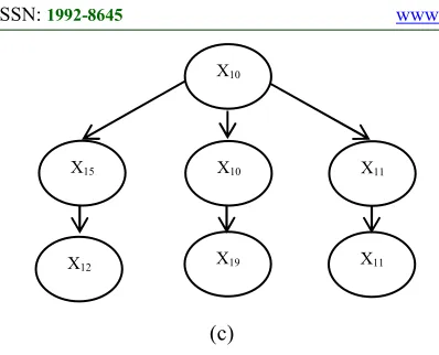
Suppose three sentences are used to express the emergence of a term taken from a dictionary term shown in Figure 2. Xi in Figure 1 will be changed by Ti according to the existence of term in each sentence on the dictionary. The joint distribution of each graph in Figure 2 can be written as # , #$, #%, #&, #' #'|#% . #%|# !.
#&|#$ . #$|# !. # for Figure 2.(a),
#(, #%, #(, # #%|#( . #(|#( .
# |#( . #( for Figure 2.(b), and
#(, #%, #(, # , # , #), # # |#% .
#%|#( . #)|#( . #(|#( . # |# .
# |#( . #( for Figure 2.(c).
(a) (b) X1
X2 X3
X1
X3
X2
X3
X2
X1
X1
X1
X4 X5
X7
X18
X10
ISSN: 1992-8645 www.jatit.org E-ISSN: 1817-3195
[image:3.612.94.293.75.236.2]255 (c)
Figure 2.DAG for three sentences
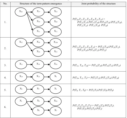
Each sentence contains some terms. The first three terms in Indonesian are generally contains the main principal of a sentence (e.g. subject, predicate, and object). Thus, in this study, these first three terms of each sentence are taken to be processed as a pattern of sentences. Algorithm 2 shows the step in constructing a dictionary of the term emergence pattern of documents.
Algorithm 2: Term emergence patterns
This algorithm would build a dictionary term emergence patterns of a master document. The steps are as follows:
• Take all appropriate term in each sentence from the term order emergence using Algorithm 1.
• Arrange those all appropriate terms follow the structure of every sentence in each document as the term emergence pattern.
• Take the first three terms from the term emergence pattern in every sentences of each document.
• Construct the joint distribution of the first three terms emergence pattern in every sentence of each document.
The emergence oftermina sentenceis always dependent on the appearance of the previous term. The series of emergence of term would construct a network of term. This network could be called as Bayesian Network due to the emergence of term series shows one come prior the other.Therefore, the series of term would represent the series of prior and posterior sequence which ensemble the Bayesian Network.
Algorithm 3 shows the steps to calculate the likelihood of the first three emergences as the joint distribution of the terms laid out in the sentence as a Bayesian Network.
Algorithm3: Likelihood of the First Three Term Emergences
This algorithm would explain how to calculate the joint probability distribution of the first three emergences of terms in every sentence as its likelihood. The steps are as follows:
• Take the first three emergences of terms from every sentence based on the term emergence pattern as representation of a sentence using Algorithm 2.
• Collect and calculate the individual term
o Collect and calculate the frequency of the
first emergences of termsfrom all sentences as a group then calculate the probability of each term amongst the first terms emergence in this group.
o Collect the second and the third emergences
of terms from all sentences and calculate their probabilities in and amongst their groups as done for the first term.
• Calculate the likelihood of each sentence by multiplying all probability of the first three emergences of terms in the sentence
The document contained some sentences, therefore, can be calculated its likelihood based on their sentence probability calculated by Algorithm 3. In addition, the principle of the sequence of sentences in such document can also be assumed as a Bayesian Network structure, but those sentences can be assumed to be independent.The probability of such pattern of document can be represented by probability of those sequences of sentences as representing in a likelihood of document calculated by multiplication of all likelihood of each sentences. When all of documents can be seen their likelihood, then they could be compared their pattern by calculating the likelihood ration of each pair documents. The algorithm to calculate the likelihood ratio between two documents can be seen in Algorithm 4.
Algorithm4: Likelihood Ratio of Document
This algorithm would explain how to calculate the likelihood ratio between two documents. The steps are as follows:
• Calculate the likelihood of each sentence represented by the first three terms in each document using Algorithm 3.
• Calculate the likelihood of each document by multiplying the likelihood of each sentence in the related document.
ISSN: 1992-8645 www.jatit.org E-ISSN: 1817-3195
256
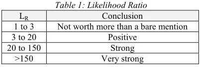
[image:4.612.93.295.152.220.2]• Decide the comparison between these two documents by using their likelihood ratio based on Bayes Factor presented in Table 1 (Kass and Raftery, 1995).
Table 1: Likelihood Ratio
LR Conclusion
1 to 3 Not worth more than a bare mention
3 to 20 Positive
20 to 150 Strong
>150 Very strong
where LR = Likelihood ratio of Doc-I and Doc-j (j≠i), for i = 1,…, k and k is the number of documents.
Algorithm 4 would be firstly applied to test the pattern similarity of five tested documents as has been used in Soehardjoepri, et.al. [1] and secondly to six documents, after one differently additional tested documents is added. The process is discussed in the following section.
4. Numerical Implementation
Five documents which has been used in Soehardjoepri, et.al. [1], are used in this section to show the work of this algorithm.Doc-1 and Doc-2 are previously designed to have an almost similar structure. Firstly, of the five documents will be peeled all their terms by using LSA as stated in Algorithm 1. The result of this algorithm is the emergence of terms in each sentence ofeach document, which are shown in Table 2.
Implementation of Algorithm 2 couple with the rule based of the first three terms inIndonesian sentences to those five documentshaving term sequence listed in Table 2, give thestructure of pattern emergence terms as shown in the second column of Table 3 to Table 7. By applying the form of Bayesian Network, the probability of the structure of each sentence is given in the third column of those tables.
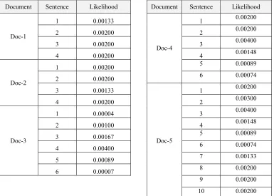
In order to find the probability of each sentence structure, Algorithm 3 could be applied. Calculation of the probability of each term in the structures has to be prepared by counting the frequency of each term occurrence which appears in every sentence of whole five documents. The frequency of each term occurrence in every sentence of five documents can be seen in Table 8. Based onthis frequency, the probability of each term occurrence can be found by calculating the related term in each appearance, as stated in the second step of Algorithm 3.By employing Table 8 and inputting it to the last step of Algorithm 3, the probability of the first three term occurrence for
each sentence in five documentsis shown in Table 9.
Comparing between two documents, e.g. Doc-1 and Doc-2 which are previously designed to have similar structure, can be done by calculating their likelihood ratios. The likelihood of each document can be calculated by employing Table 9 and inputting it to Algorithm 4. Supposing that the Doc-1 is more preferable than Doc-2, the likelihood ratio can be found by dividing likelihood of Doc-1 with likelihood of Doc-2. Where based on Table 9, the likelihood of Doc-1 and Doc-2 are 0.1 x 10 ( respectively. Therefore, the likelihood ratio is 1 and do not reject the null hypothesis (e.g. Doc-1 and Doc-2 have similar structure).
ISSN: 1992-8645 www.jatit.org E-ISSN: 1817-3195
257
Table2: The Emergence Oftermsineach Sentenceof Each Document (Doc)
Docu ment
Senten ce
Occurrence order
1 2 3 4 5 6 7 8 9 10
Doc-1
1 T19 T2 T1
2 T9 T7 T1 T2 T1 T3
3 T1 T4 T18 T9 T8 T6 T2
4 T1 T5 T7 T2 T18 T6 T2 T5 T4 T3
Doc-2
1 T1 T4 T18 T9 T8 T6 T2
2 T1 T5 T7 T2 T18 T6 T2 T5 T4 T3
3 T19 T2 T1
4 T9 T7 T1 T2 T1 T3
Doc-3
1 T17 T12 T10 T16 T15 T11 T10
2 T10 T15 T12
3 T10 T10 T19
4 T10 T11 T11
5 T13 T14 T11 T10 T16
6 T13 T13 T14 T12 T12
Doc-4
1 T10 T17 T12 T17 T16 T15 T11 T10
2 T12 T10 T15
3 T10 T19 T10
4 T10 T11 T11
5 T11 T10 T16 T14 T13
6 T12 T14 T13 T12 T13
Doc-5
1 T10 T17 T12 T17 T16 T15 T11 T10
2 T12 T10 T15
3 T10 T19 T10
4 T10 T11 T11
5 T11 T10 T16 T14 T13
6 T12 T14 T13 T12 T13
7 T19 T12 T1
8 T9 T7 T1 T2 T1 T3
9 T1 T4 T18 T9 T8 T8 T6 T2
ISSN: 1992-8645 www.jatit.org E-ISSN: 1817-3195
[image:6.612.86.521.289.456.2]258
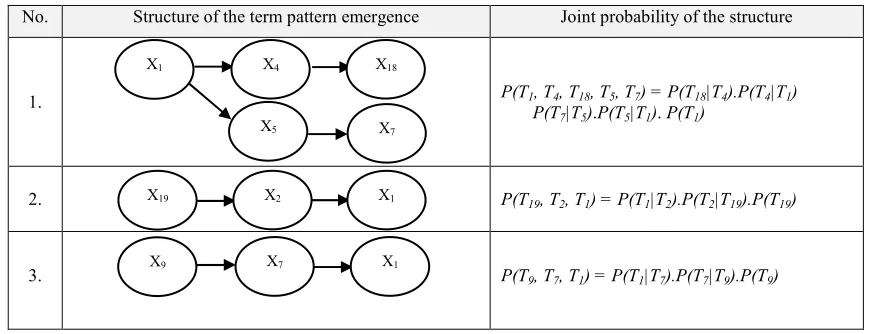
Table 3: Structure Of The Term Pattern Emergence And Its Probability For Doc-1
Structure of the term pattern emergence Joint probability of the structure
1. P(T19, T2, T1) = P(T1|T2).P(T2|T19).P(T19)
2. P(T9, T7, T1) = P(T1|T7).P(T7|T9).P(T9)
3. P(T1, T4, T18, T5, T7) = P(T18|T4).P(T4|T1)
P(T7|T5).P(T5|T1). P(T1)
Table 4: Structure Of The Term Pattern Emergence And Its Probability For Doc-2
No. Structure of the term pattern emergence Joint probability of the structure
1. P(T1, T4, T18, T5, T7) = P(T18|T4).P(T4|T1)
P(T7|T5).P(T5|T1). P(T1)
2. P(T19, T2, T1) = P(T1|T2).P(T2|T19).P(T19)
3. P(T9, T7, T1) = P(T1|T7).P(T7|T9).P(T9)
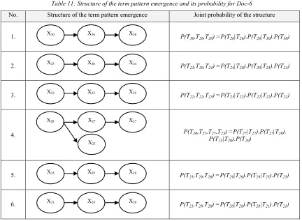
To show the work of this proposed method, we take another document (called Doc-6) which is designed as almost similar to documents five but it is designed as totally different with the four previous documents. After LSA has succeeded to process all of six documents and applying Algorithm 1 followed by cutting the first three terms of them, then the term emergence patterns of Doc-6 is shown in Table 11.
The frequency of each occurrence of the term in every sentence of the six documents can be seen in Table 12, revising the information in Table 8. Based on the frequency in Table 12 and applying Algorithm 3, the likelihood of each sentence in every document for all of six documents would be
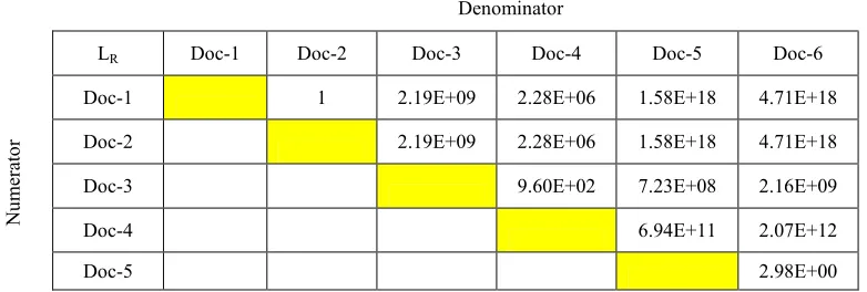
changed from Table 9 to Table 13. The pairwise likelihood ratio amongst the six documents, therefore, can be found by applying Algorithm 4 and the result can be seen in Table 14.
Based on Table 14, the testing to similarity pattern of Doc-6 to those previous five documents will not change the previous decision amongst the previous five documents. This table also shows the prove that Doc-6 is significantly different with all of documents except between Doc-5 and Doc-6. These last two documents have almost similar pattern, due to their likelihood ratio that can be stated as ‘Not worth more than a bare mention’ as in Table 1.
X19 X2 X1
X9 X7 X1
X1 X4 X18
X5 X7
X1 X4 X18
X5 X7
X19 X2 X1
ISSN: 1992-8645 www.jatit.org E-ISSN: 1817-3195
[image:7.612.90.523.79.328.2]259
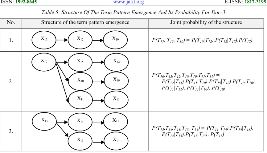
Table 5: Structure Of The Term Pattern Emergence And Its Probability For Doc-3
No. Structure of the term pattern emergence Joint probability of the structure
1. P(T17, T12, T10) = P(T10|T12).P(T12|T17).P(T17)
2.
P(T10,T15,T12,T10,T19,T11,T11) =
P(T12|T15).P(T15|T10).P(T19|T10).P(T10|T10).
P(T11|T11). P(T11|T10). P(T10)
3. P(T13,T14,T11,T13, T14) = P(T11|T14).P(T14|T13).
[image:7.612.87.521.365.582.2]P(T14|T13).P(T13|T13). P(T13)
Table 6: Structure Of The Term Pattern Emergence And Its Probability For Doc-4
No. Structure of the term pattern emergence Joint probability of the structure
1.
P(T10,T17,T12,T19,T10,T11,T11) =
P(T12|T17).P(T17|T10).P(T10|T19).P(T19|T10).
P(T11|T11). P(T11|T10). P(T10)
2. P(T12,T10,T15,T14,T13) = P(T15|T10).P(T10|T12).
P(T13|T14).P(T14|T12).P(T12)
3.
P(T11, T10, T16) =P(T16|T10).P(T10|T11).P(T11)
X17 X12 X10
X10 X15 X12
X10 X19
X11 X11
X13 X14 X11
X13 X14
X10 X17 X12
X19 X10
X11 X11
X12 X10 X15
X14 X13
ISSN: 1992-8645 www.jatit.org E-ISSN: 1817-3195
[image:8.612.90.521.103.502.2]260
Table 7: Structure of the term pattern emergence and its probability for Doc-5
No. Structure of the term pattern emergence Joint probability of the structure
1.
P(T10,T17,T12,T14,T10,T11,T11) =
P(T12|T17).P(T17|T10).P(T10|T14).P(T14|T10).
P(T11|T11). P(T11|T10). P(T10)
2. P(T12,T10,T15,T14,T13) = P(T15|T10).P(T10|T12).
P(T13|T14).P(T14|T12).P(T12)
3. P(T11, T10, T16) = P(T16|T10).P(T10|T11).P(T11)
4. P(T19, T12, T1) = P(T1|T12).P(T12|T19).P(T19)
5. P(T9, T7, T9) = P(T1|T7).P(T7|T9).P(T9)
6. P(T1,T4,T18,T5,T7) = P(T18|T4).P(T4|T1).
P(T7|T5).P(T5|T1).P(T1)
Table 8: The frequency of term occurrence in five documents
Occurrence Sequence
1st 2nd 3rd
Ter
m Freq Term Freq Term Freq
T10 9 T10 5 T1 6
T1 6 T7 3 T11 4
T12 4 T4 3 T18 3
T9 3 T5 3 T7 3
T19 3 T11 3 T10 3
T11 2 T14 3 T12 3
T13 2 T2 2 T15 2
T17 1 T12 2 T16 2
T17 2 T13 2
T19 2 T19 1
T15 1 T14 1
T13 1
X10 X17 X12
X14 X10
X11 X11
X12
X14
X10 X150
X13
X11 X10 X16
X19 X12 X1
X9 X7 X1
X1
X5
X4 X18
[image:8.612.221.393.531.723.2]ISSN: 1992-8645 www.jatit.org E-ISSN: 1817-3195
[image:9.612.162.467.172.283.2]261
Table 9: Likelihood Of Each Sentence In Each Document
Table 10: Likelihood ratiosfor pair ways of 5documents
Document Sentence Likelihood Document Sentence Likelihood
Doc-1
1 0.00133
Doc-4
1 0.00200
2 0.00200 2 0.00200
3 0.00200 3 0.00400
4 0.00200 4 0.00148
Doc-2
1 0.00200 5 0.00089
2 0.00200 6 0.00074
3 0.00133
Doc-5
1 0.00200
4 0.00200 2 0.00300
Doc-3
1 0.00004 3 0.00400
2 0.00100 4 0.00148
3 0.00167 5 0.00089
4 0.00400 6 0.00074
5 0.00089 7 0.00133
6 0.00007 8 0.00200
9 0.00200
10 0.00200
Denominator
LR Doc-1 Doc-2 Doc-3 Doc-4 Doc-5
N
u
m
er
at
o
r
Doc-1
1 6.01E+08 6.41E+06 4.02E+16
Doc-2
6.01E+08 6.41E+06 4.02E+16
Doc-3
9.37E+01 6.69E+07
Doc-4
[image:9.612.116.501.426.701.2]ISSN: 1992-8645 www.jatit.org E-ISSN: 1817-3195
[image:10.612.89.521.94.411.2]262
Table 11: Structure of the term pattern emergence and its probability for Doc-6
No. Structure of the term pattern emergence Joint probability of the structure
1. P(T30,T26,T26) =P(T26|T26).P(T26|T30).P(T30)
2. P(T23,T20,T24) =P(T24|T20).P(T20|T23).P(T23)
3. P(T22,T22,T25) =P(T25|T22).P(T22|T22).P(T22)
4. P(T20,T27,T27,T23) =P(T27|T27).P(T27|T20).
P(T23|T20).P(T20)
5. P(T25,T29,T29) =P(T29|T29).P(T29|T25).P(T25)
6. P(T21,T28,T20) =P(T20|T28).P(T28|T21).P(T21)
[image:10.612.92.596.445.714.2]Table12: The frequency of term occurrence in six documents
Table 13: Likelihood Of Each Sentence In Each Document Occurrence Sequence
1st 2nd 3rd
Term Freq Term Freq Term Freq
T10 9 T10 5 T1 6
T1 6 T7 3 T11 4
T12 4 T4 3 T18 3
T9 3 T5 3 T7 3
T19 3 T11 3 T10 3
T11 2 T14 3 T12 3
T13 2 T2 2 T15 2
T17 1 T12 2 T16 2
T20 2 T17 2 T13 2
T30 1 T19 2 T19 1
T25 1 T15 1 T14 1
T23 1 T13 1 T26 1
T22 1 T26 1 T24 1
T21 1 T20 1 T25 1
T22 1 T27 1
T27 1 T29 1
T29 1 T20 1
T23 1
T28 1
Docu
ment Sentence Likelihood
Docu
ment Sentence Likelihood
Doc-1
1 0.00073
Doc-5
1 0.00110
2 0.00110 2 0.00164
3 0.00110 3 0.00219
4 0.00110 4 0.00081
Doc-2
1 0.00073 5 0.00049
2 0.00110 6 0.00110
3 0.00110 7 0.00110
4 0.00110 8 0.00041
Doc-3
1 0.00002 9 0.00073
2 0.00055 10 0.00110
3 0.00091
Doc-6
1 0.00002
4 0.00219 2 0.00002
5 0.00049 3 0.00002
6 0.00004 4 0.00004
Doc-4
1 0.00041 5 0.00146
2 0.00110 6 0.00002
3 0.00110 7 0.00002
4 0.00219
5 0.00081
6 0.00049
X30 X26 X26
X23 X20 X24
X22 X22 X25
X25 X29 X29
X21 X28 X20
X20
X23
ISSN: 1992-8645 www.jatit.org E-ISSN: 1817-3195
[image:11.612.116.507.115.247.2]263
Table 14: Likelihood Ratiosfor Pair Ways Of Six Documents
Denominator
LR Doc-1 Doc-2 Doc-3 Doc-4 Doc-5 Doc-6
N
u
m
er
at
o
r
Doc-1 1 2.19E+09 2.28E+06 1.58E+18 4.71E+18
Doc-2
2.19E+09 2.28E+06 1.58E+18 4.71E+18
Doc-3 9.60E+02 7.23E+08 2.16E+09
Doc-4 6.94E+11 2.07E+12
Doc-5 2.98E+00
6. CONCLUSIONS
Finally it can be concluded that the Latent Semantic Analysis, Bayesian Network and Likelihood Ratio which are structured in four algorithms in this paper strongly able to identify pattern similarities term emergence of two documents.
7. ACKNOWLEDGEMENT
The authors thank BPPDN-College which has provided scholarships for doctoral programs and the Department of Statistics Institute of Technology (ITS) which provide facilities, giving a boost to publish in international journals and motivate doctoral program is immediately resolved. Thanks also to the anonymous reviewer who has reviewed this paper.
REFERENCES:
[1] Soehardjoepri, Iriawan, N., Ulama, B.S.S., and Irhamah, “On the Text Documents Pattern Recognition Using Latent Semantic Analysis and Kolmogorov-Smirnov Test”, South East Asian Conference on Mathematics and Its Applications, Department of Mathematics, FMIPA-ITS, Surabaya-Indonesia, 2013.
[2] Landauer, T.K., Foltz, P.W., and Laham, D., “Introduction to Latent Semantic Analysis”, Discourse Processes, 25 (1998), 259 - 284. [3] Kevin, B.K. and Ann, E.N., “Bayesian
Artificial Intelligence Second Edition”, Computer Science and Data Analysis Series, CRC Press, New York, 2011
[4] S.K.M. Wong and C.J. Butz, “A Bayesian Approach to User Profiling in Information Retrieval”, Saskatchewan, Canada, S4S 0A2 Ottawa, Ontario, Canada, K1N 6N5, 2000.
[5] C.K. Chow and C.N. Liu, “Approximating discrete probability distributions with dependence trees”, IEEE Transactions on Information Theory, IT-14, 3, 462-467, 1968.
[6] Kass R.E. and Raftery, A.E., “Bayes Factors”, Journal of the American Statistical Association, Vol.90, No. 430 (Jun., 1995), 773-795.
[7] Ben-Gal I., “Bayesian Networks”, in Ruggeri F., Faltin F. &Kenett R., Encyclopedia of Statistics in Quality & Reliability, Wiley & Sons, 2007.
[8] Soehardjoepri, Iriawan, N., Ulama, B.S.S., and Irhamah, ”Identifying Text Document Pattern For Two Terms Appearances VIA Latent Semantic Analysis (LSA) Method And Term Distance Between Two Documents”, Journal of Theoretical and Applied Information Technology, 20th September 2015. Vol.79. No.2, 322 – 329, ISSN: 1992-8645, E-ISSN: 1817-3195, JATIT & LLS, Pakistan, 2015.
[9] Pawan G., Laxmidhar B. and T.M. McGinnity, “Application of Bayesian Framework in Natural Language Understanding”, Vol.25, ISSUE 2008, 251 – 269, IETE TECHNICAL REVIEW, doi: 10.4103/0256-4602.44656.
[10] Ozgur, L., and Gungor, T., “Text classification with the support of pruned dependency patterns”, Elsevier B.V, 1598–
1607, 2010,
doi:10.1016/j.patrec.2010.05.005.
[11] Ghanem, M., Guo, Y., Lodhi, H., and Zhang, Y., “Automatic scientific text classification using local patterns”, ACM SIGKDD Explore News. 4 (2), 95–96, 2002.
ISSN: 1992-8645 www.jatit.org E-ISSN: 1817-3195
264 Technology 38: 188 (2005), doi: 10.1002/aris.1440380105.
[13] Deerwester, S., Dumais, S.T., Landauer, T., Furnas, G. and Harshman, R, “Indexing by Latent Semantic Analysis”, Journal of the American Society of Information Science 41, (6): 391- 407, 1990.
[14] Thomas L., Peter W. F., and Darrell L., “Introduction to Latent Semantic Analysis”, Discourse Processes 25, 259-284, 1998, doi: 10.1080/01638539809545028.
[15] Law, A. M., and Kelton, W. D., “Simulation Modeling and Analysis”, McGraw-Hill International Series, Singapore, 2000. [16] Thomas L., Peter W. F., and Darrell L.,
“Introduction to Latent Semantic Analysis”, Discourse Processes25, 259-284, 1998, doi: 10.1080/01638539809545028.
[17] Kasim, S.,