BIROn - Birkbeck Institutional Research Online
Northcott, Robert (2012) Degree of explanation. Synthese , ISSN
0039-7857.
Downloaded from:
Usage Guidelines:
Please refer to usage guidelines at or alternatively
BIROn
-
B
irkbeck
I
nstitutional
R
esearch
On
line
Enabling open access to Birkbeck’s published research output
Degree of explanation
Journal Article
http://eprints.bbk.ac.uk/4995
Version: Accepted (Refereed)
Citation:
© 2012 Springer
Publisher Version
______________________________________________________________
All articles available through Birkbeck ePrints are protected by intellectual property law, including copyright law. Any use made of the contents should comply with the relevant law.
______________________________________________________________
Deposit Guide
Contact: [email protected]
Birkbeck ePrints
Birkbeck ePrints
Northcott, R. (2012)
Degree of explanation
Degree of Explanation
Abstract
Partial explanations are everywhere. That is, explanations citing causes that explain some but not all of an effect are ubiquitous across science, and these in turn rely on the notion of degree of explanation. I argue that current accounts are seriously deficient. In
particular, they do not incorporate adequately the way in which a cause’s explanatory importance varies with choice of explanandum. Using influential recent contrastive theories, I develop quantitative definitions that remedy this lacuna, and relate it to existing measures of degree of causation. Among other things, this reveals the precise role here of chance, as well as bearing on the relation between causal explanation and causation itself.
1) Introduction
One of the central aims of the sociological classic Bowling Alone (Putnam 2000) is to identify the causes of the decline in ‘social capital’ in the USA since 1960. Many candidates have been suggested: increased work hours; suburban sprawl; government welfare policy; more women going to work; television; increased divorce rates; and others besides. It turns out (Putnam argues) that no single cause explains the decline entirely. The question of critical interest, both historically and as a guide to future intervention, is to quantify each cause’s partial contribution. The focus is not on how general or deep or transportable a particular explanation or mechanism is, important though those concerns may also be, but rather is narrowly on the extent to which a cause explains an effect in a specific singular case. A singular explanation may well be derived from a generalization; nevertheless, its accuracy in a specific case is a distinct issue.
To repeat, in this and other cases no individual cause explains all of the explanandum. So our philosophical task is not to assess which among several complete or full explanations is preferable; rather, it is to assess the extents to which different incomplete explanations are incomplete in a single case.1 Why should we be motivated to analyze degree of explanation, so understood? Because this issue arises ubiquitously in both science and everyday life. How much was the decreased murder rate explained by lower
unemployment? Which was the more important cause of the plant’s height, the fertilizer or the new greenhouse? Was it the penetrating offense or the stout defense that was mainly responsible for the football team’s victory? The relevant explanations here are acknowledged by all to be incomplete; the concern is rather to what degree each explained their explanandum.
Such judgments are made implicitly all the time but they require conceptual clarification. Comparing different causes’ importance, and apportioning responsibility between them, requires making good sense of the notion of partial explanation, i.e. of degree of
explanation.2 A quantitative notion of degree of causation is already widespread in
1
It might be that the measures to be developed in this paper can be applied to type-level explananda too. But I will frame the discussion in terms of token cases only.
2
statistics and many sciences. And the problem of explanandum-dependence (to be discussed below) is also widely recognized. But, I will argue, the latter issue implies problems for the standard view of the former, and this has not been widely recognized, thus motivating the need to develop a definition specifically of degree of explanation.
It turns out to be very useful to make our concepts in this area explicit. For instance, if the causes in a partial explanation are probabilistic, how much is the outcome due to them and how much to simple chance? Should a definition incorporate both aspects? Can they even be separated? What is the role of contrasts? The devil is in the details.
I frame the analysis in terms of a contrastive-counterfactual theory of causal explanation, in accordance with current philosophical orthodoxy. As Ylikoski and Kourikoski (2010) comment, this ties together theoretical and practical knowledge, because explanatory understanding can now be cashed out in the currency of advice regarding interventions. In particular, degree of explanation will by definition capture the extent to which an intervention is the one we want. More precisely, it will capture the amount by which the impact of the intervention licensed by a partial explanation falls short of the desired impact. It also answers what-if-things-had-been-different questions by expressing the extent to which things would have been as different as we wanted them to be.
The formal task turns out to be a delicate one. The vast literature on defining causation itself is of no direct help because in the cases of interest here typically all parties already agree on what causes are present. The issue at hand is, rather, each cause’s explanatory importance, and this matter of degree is clearly distinct from mere causation or
explanation simpliciter. To be clear: the issue is not that existing theories of causation and explanation are incorrect. Indeed, as noted, this paper’s analysis will be framed in terms of existing difference-making views. Rather, the issue is that there is an unfulfilled need to use these theories to define degree of explanation precisely. Structural equations, for instance, can certainly be used to motivate the definitions of degree of explanation that I develop, and to calculate the quantities that enter those definitions. However, they do not furnish the definitions themselves.
Although the issues here are of great applied import, this paper is a theoretical one. It is organized as follows: I begin by stating a familiar quantitative definition of degree of causation (section 2). I then introduce the problem of explanandum-dependence, to motivate the need for a separate definition specifically of degree of explanation (section 3). Sections 4 to 8 are devoted to the intricate task of chiseling out such a definition. I then finish by exploring that definition’s relation to previous work (section 9), and its implications for the distinction between causation and explanation (section 10).
2) Causal strength
Let X be a cause variable and Y an effect variable. Y is a function of the state of the world, i.e. of X and W, where W is background conditions (i.e. formally a set of variables representing the state of the world just excluding X).3 Let XA denote the actual value of
X, and XC the salient counterfactual value of X. And letYA and YC denote the values that
3
Y takes given XA and XC respectively.4 Then define the degree of causation (or,
equivalently, the causal strength or importance) of a cause variable X with respect to an effect variable Y, to be:
Y
A– Y
C[1]
Formula [1] is quite intuitive, being just a representation of counterfactual difference-making. We are interested in the quantity of effect for which XA is responsible, and this is
just the level of effect with XA compared to the level with the alternative input XC. The
unit of any CS is the unit of the effect variable Y. The actual and counterfactual values of Y are real numbers. A causal strength (‘CS’) is the difference between them, and may be positive, zero or negative. For example, the CS of kicking a ball might be yielded by the ball’s acceleration with the kick compared to its acceleration without that kick.5
A negative CS here would correspond to accelerating the ball backwards; a zero CS to leaving its acceleration unchanged.
At the heart of [1] is that it captures a controlled-experiment sensibility. We want to compare the level of effect with and without the cause while keeping all else equal. For instance, it would be no use comparing the acceleration of a ball with and without a kick if simultaneously a gust of wind had blown up, because obviously the calculation would then yield only the combined impact of the two changes. For this reason, the terms in [1] must be evaluated with the background conditions constant across the two terms.6
YC, the right-hand term in [1], is a counterfactual – we are interested in what the level of
effect would have been, given XC and W. How can this term be evaluated? Because, in
reality, background conditions are never quite exactly the same from moment to moment, epistemologically the best we can ever do is find data from as good a re-creation as possible of the relevant conditions. In this respect, [1] serves as a normative ideal, telling us what hypothetical quantity is relevant to evaluating a CS. Only some actual sources of data, namely those adequately approximating controlled constant-W conditions, will then be appropriate.7
3) The problem of explanandum-dependence
Not surprisingly, [1] or something like it has a long history in several different literatures as a measure of degree of causation. In the philosophy of history, the motivation behind
4
For ease of exposition, as well as using YA, XC etc to denote particular values of a variable, throughout I will also use them to denote particular events that instantiate those values. I will reserve lower-case notation, i.e. yA, xC etc, for values of qualitative variables (section 5 below).
5
Often, as with temperature, the ‘absence’ of a cause may make little sense. Rather, in such cases we are interested in the impact of a cause relative to some specific non-zero alternative. Thus when occasionally I refer to the absence or negation of a cause this should be understood merely as convenient shorthand for some salient XC. No commitment is implied to ‘negative events’.
6
Strictly speaking, in fact the background conditions are not constant because as well as impacting Y, in general a change from XC to XA will also change W too. But for our purposes we may ignore that wrinkle, so long as any change in W is only a consequence of the change in X. The point is that incorporating a counterfactual term and conditioning on W eliminates spurious correlations.
7
[1] is similar to that behind several classical views, for instance those in the nineteenth century of Yule and Weber (Turner 1986, Northcott 2008c). More recently, measures in psychology, psychiatry, statistics, epidemiology, law and computer science are similar. Moreover, still other measures are closely related, being again essentially comparative of an effect with and without a cause.
Within analytic philosophy, [1] reflects the common emphasis on causation’s difference-making aspect – a cause is something that makes a difference to its effect. Thus,
naturally, the strength of a cause is how much difference it makes. The form of [1] can be incorporated into the contemporary Bayes net and causal modeling literatures, and
arguably is endorsed by experimental practice, at least in the case of quantitative variables (Woodward 2003, Pearl 2000, Spirtes et al 2000). More generally, it is also consistent with the mainstream literature on probabilistic causation (Hitchcock 1996).
Yet, notwithstanding this ubiquity, [1] cannot yet be a complete account of degree of
explanation. The reason stems from the fact that contemporary theories of causal
explanation are contrastive in both the cause and effect slots (Dretske 1972, Van Fraassen 1980, Garfinkel 1981, Achinstein 1983, Woodward 2003).8 On this view, explanation takes the general form:
XA-rather-than-XC explains YA-rather-than-YC
where YA and YC are respectively the actual and contrast values of the effect variable Y.
Intuitively, this captures the sensitivity of explanation to the precise specification of the explanandum. As it were, YC picks out which aspect of the effect is of interest, and
without it an explanandum is under-specified.
As (Sober et al 1992, 134) remarks: “A problem that constantly befuddles debates about the importance of different causes … is the correct designation of the object of
explanation (the explanandum)”. (Sober et al 1992) and (Martin 1989) are two of the few to emphasize it in this context.
The problem – for everyone – is that formula [1] is vulnerable on exactly this point. In particular, it incorporates choice of contrast only on the cause side, which is fine for an analysis of CS but not for one of degree of explanation. With regard to the latter, [1] stands incomplete. Although the contrastive view of explanation neatly captures
explanandum-dependence, no one (to my knowledge) has ever adapted its machinery to the issue of defining degree of explanation. This is a notable lacuna.
To make matters more precise, begin by noting that any contrastive explanandum takes the form ‘YA-rather-than-YC’, where YA and YC are values of the effect variable Y. Now
introduce a subtle but important point of notation. So far, we have defined YA and YC to
be the values that Y takes when X = XA and X = XC respectively. However, these YA and
YC are not necessarily the ‘YA’ and ‘YC’ that characterize a target explanandum.
Therefore, for clarity, I will henceforth denote a target explanandum instead by YA
*-rather-than-YC*. The asterisks signify that these particular values of Y are specified
8
independently of any particular explanans, i.e. independently of any particular values of X. There is no guarantee that YA and YC will match precisely YA* and YC*. The crucial
matter, as we will see, is the extent to which they indeed do.
[1]’s critical insensitivity is to these YC* and YA*. There is of course a sense in which [1]
is perfectly ‘sensitive to YC’ already, namely that its right-hand term is by definition a
contrast level of Y. The key point though is that [1]’s ‘YC’ is a function of the explanans,
in particular of XC; yet this is not the ‘YC’ that [1] needs to be sensitive to, which is that
one specified by the explanandum independently of the explanans, i.e. YC*. Analogous
points apply to [1]’s incorporation of YA instead of YA*. Fundamentally, the problem is
really [1]’s insensitivity to choice of explanandum, i.e. to both YC* and YA*. The result is
that we still have no acceptable account of degree of explanation.
All this becomes clearer by example. Take, for instance, the first dropping of an atomic bomb in war. What explains the timing of this event? In other words, why did it occur on 6th August 1945 at Hiroshima? Consider two causes: the fine weather that day; and Japan’s reluctance to surrender. And respective salient contrasts: bad weather that day; Japan amenable to surrender. Both these causes can be argued to have greatly increased the bombing’s probability. First, if the weather had been bad instead of good, the bombing would have been postponed.9 Second, if Japan had been willing to surrender, Truman would likely have thought the bombing unnecessary. But the two causes increase the probability of different aspects of the bombing. In particular, the weather impacted its precise timing, whereas the Japanese attitude impacted only its rough timing (or, for those optimists who believe that there might otherwise never have been such an event, whether a first atomic bombing occurred at all). Thus the weather is highly explanatory of the short-term explanandum – why the first bombing occurred on 6th August 1945 rather than in the subsequent few days (i.e. YC* = the bomb was first dropped in the
subsequent few days); Japan’s attitude, by contrast, is highly explanatory of a longer-term explanandum – why the first bombing occurred in 1945 rather than in some subsequent year (i.e. YC* = the bomb was first dropped only in subsequent years).
The problem is that the simple formula [1] is unable to capture this crucial distinction. Both the weather and the Japanese attitude made a big difference to whether the bomb was dropped, and for this reason both factors score well on [1]. But it is impossible to represent in [1] the crucial distinction between the long-run and short-run explananda, because just considering YA and YC alone still leaves unclear which aspect of the effect is
explanatorily relevant. In the notation of this paper, we need a successor to [1] that is YC*-sensitive.
Might, though, the difference between the two explananda be representable in [1] after all, in particular via a judicious choice of effect variable? Let us see why not. The suggestion is that we can incorporate appropriate sensitivity to YC* indirectly via our
definition of Y. For instance, we might invoke the longer-term explanandum by defining
9
Y in a coarse-grained manner, say delineating time by year. Then YA* = the bomb was
dropped in the year 1945. Sure enough, this generates, as desired, a high causal strength for Japan’s attitude but not for the weather. Formally, applying a probabilistic version of [1]10, and simplifying the relevant probabilities to 1 and 0:
-- Weather’s causal strength = pr(a bomb was first dropped in 1945 / fine weather on 6th August 1945) – pr(a bomb was first dropped in 1945/ bad weather on 6th August 1945) = 1 – 1 = 0
-- Japan’s attitude’s causal strength = pr(a bomb was first dropped in 1945 / Japan’s actual attitude) – pr(a bomb was first dropped in 1945 / Japan amenable to surrender) = 1 – 0 = 1
So far, so good. But how do we apply the same strategy to the short-run explanandum? Presumably Y would now have to be fine-grained, so that YA* = a bomb was first
dropped on 6th August 1945 precisely. Running through the calculations for this new YA*:
-- Weather’s causal strength = pr(a bomb was first dropped on 6th August 1945 / fine weather on 6th August 1945) – pr(a bomb was first dropped on 6th August 1945 / bad weather on 6th August 1945) = 1 – 0 = 1
-- Japan’s attitude’s causal strength = pr(a bomb was first dropped on 6th August 1945 / Japan’s actual attitude) – pr(a bomb was first dropped on 6th
August 1945 / Japan amenable to surrender) = 1 – 0 = 1
The problem is the second calculation: the Japanese unwillingness to surrender still scores highly even for the short-run explanandum. Indeed, it is hard to see how this can be avoided if, like [1], we take no consideration of YC*. For (focusing on the right-hand
terms in each calculation) what would be required, roughly speaking, is a true description of the Hiroshima bomb drop that was sufficiently fine-grained to be rendered improbable by bad weather yet also sufficiently coarse-grained to be rendered probable by Japanese willingness to surrender. It seems impossible to satisfy both these constraints
simultaneously.
Similar dilemmas arise in many other examples. I conclude that, when formulating degree of explanation, [1] alone cannot be enough. Yet the problem can be solved, as we will see, by a formula that incorporates explicitly the explanandum values of Y, i.e. YA*
and YC*.
4) Degree of explanation I – the quantitative case
As it will be understood here, degree of explanation (‘DE’) is an objective relation in a token case between an explanandum and an explanans. The sequence of analysis will be as follows:
-- First, we define a target explanandum YA*-rather-than-YC*, i.e. an actual value YA*
and contrast value YC* of the effect.
-- Second, we consider an explanans XA-rather-than-XC, i.e. an actual value XA and
contrast value XC of a cause. This explanans automatically yields suggested values for
YA* and YC*, namely YA and YC.
10
-- Then third, we compare the target explanandum values of the effect variable with those values suggested by the explanans, i.e. we compare YA* with YA, and YC* with YC. DE
is then a matter of how well the explanans’s suggested values for Y match up with the target ones.
It may help intuition to compare degree of explanation DE, so conceived, with causal strength CS. Consider interventions: the CS definition [1] tracks the impact of these directly. In particular, it tracks the impact on Y of a change from XC to XA. But things are
not quite the same with DE. Rather, we can think of DE instead in terms of the desired
result of an intervention. In particular, DE tracks how well a change from XC to XA will
yield the desired change from YC* to YA*. That is, CS tracks the impact of an
intervention; DE tracks to what extent this impact is the one we wanted.
Making our understanding of DE precise will be the (surprisingly intricate) business of the next few sections. Begin with cases where the effect and effect-contrast are different values of the same quantitative or scalar variable. Perhaps, say, the explanandum is why something is one height rather than another, or one temperature rather than another. Formally, such an explanandum can be represented by YA*-rather-than-YC* for some
quantitative variable Y. A critical initial question is then: given W, would a change from XC to XA be responsible for exactly the salient change from YC* to YA*? If so, then I
deem XA-rather-than-XC to be fully explanatory.
This latter term deserves explication. For, sowing confusion, ‘full explanation’,
‘explanatory strength’, ‘explanatory power’ and the like can mean many different things (see Ylikoski and Kuorikoski 2010 for a survey). So, to be clear: the sense of ‘fully explanatory’ that I have in mind is when a cause makes all (rather than only some of) the difference with respect to an effect. This is the sense that is of critical interest when considering interventions and thus the one that dovetails best with contemporary theories of causal explanation. This is also the sense that dovetails with our starting desideratum, as the ‘partial explanations’ I wish to illuminate are those that specify a cause that makes only some of the difference – and not explanations that are ‘partial’ merely in the sense of specifying only one cause out of the many that determine any given event.
More generally, the implicit alternative definition here is that we have ‘full explanation’ only when we have an accurate description of all an event’s causes. But this seems pointlessly to insist on an unattainable perfection, and in practice would render no explanation anything other than ‘partial’. As noted, a difference-making view of causal explanation naturally lends support instead to describing as ‘fully’ explanatory any cause that makes all the difference; what else, on a difference-making view, could full
explanation be?
More formally, then, in the sense just specified, XA-rather-than-XCfully explains YA
*-rather-than-YC* if and only if the following two conditions are both satisfied:
1) YA = YA*, i.e. YA* occurs when XA occurs
2) YC = YC*, i.e. YC* would have occurred had XC occurred
Our true goal, however, is a measure of partial explanation. We may now define this as how close we come to satisfying the conditions for full explanation. Formally, the degree of explanation of an explanans XA-rather-than-XC with respect to an explanandum YA
*-rather-than-YC* is:
|Y
A* – Y
A| + |Y
C* – Y
C|
[2]
Intuitively, [2] captures the distance between the target levels of Y and the levels of Y suggested by the explanans.11 For this reason, the smaller [2]’s value the better the DE. We have full explanation if and only if [2]’s value is zero, which follows only if the two conditions for full explanation earlier are both satisfied. The DE score corresponding to the neutral case of no explanation is typically |YA* – YC*|, i.e. the size of the starting
explanandum.12 As with formula [1], constant background conditions are assumed. The units of DE are the units of the effect variable Y.
To accommodate indeterminism, we should interpret YA and YC to be expected values.
Thus, strictly, [2] should be: E(|YA* – YA|) + E(|YC* – YC|). But for ease of exposition, in
the text I will omit explicit reference to the expected-value operators. I discuss
indeterminism more in the next section. (In the deterministic case, necessarily YA* = YA
and so [2] reduces to its right-hand term.)
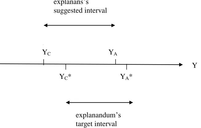
Visually, imagine a line representing the Y-variable, and compare two intervals defined on that line as per Figure 1 – the target explanandum interval [YA*, YC*] and the interval
suggested by the explanans [YA, YC]. DE is then a matter of how well the suggested
interval matches the target one. (CS corresponds to the suggested interval alone.) The left-hand term in [2] corresponds to the horizontal distance between points YA* and YA;
the right-hand term to that between YC* and YC. In the case of full explanation, both the
distances are zero.
(INSERT FIGURE 1 HERE)
A focus on actual events alone cannot capture DE satisfactorily. To see why the right-hand term in [2] is necessary, suppose we wish to explain why the tea in a cup is 23 rather than 0 degrees Celsius, i.e. is room temperature rather than freezing. Then YA* =
23 and YC* = 0. And suppose further we offered up a clearly irrelevant explanans such as
‘because my team won rather than lost the ballgame last night’. Then YA, i.e. the
temperature of the tea given that my team won the game, is room temperature, i.e. 23 degrees. It follows that the left-hand term in [2], |YA* – YA|, is zero, just as desired. The
11
Absolute values appear in the formula because it is the absolute size of the distance, rather than its direction, that matters. We thereby also avoid the undesirable possibility of two non-zero terms cancelling each other out.
12
obvious explanatory inadequacy only shows up in the counterfactual right-hand term, because even if my team had lost the ballgame, still the tea would have been room temperature anyway. Thus YC = 23 too, and so the right-hand term in [2], |YC* – YC|,
becomes |0 – 23|. Therefore [2]’s overall value is also |0 – 23|, i.e. precisely the size of the starting explanandum, and nothing has been gained. In conclusion, on any contrastive view we must consider more than actual events. The critical fact here is that the result of the ballgame made no difference, but this was not revealed by the left-hand term alone.
5) Degree of explanation II – the qualitative case
Turn next to perhaps the most common case, namely when the effect variable is
qualitative, for instance if the effect of interest is a discrete event. Examples include: the dropping of the Hiroshima bomb, the American Revolution, or a leaf having a particular color. Even though ultimately I will argue that the qualitative and quantitative cases are closely related (section 7), it will still prove useful to distinguish them notationally. So for qualitative effect variables, switch to the lower case, letting yA* denote the target
effect event and yC* denote the target contrast effect event. Note from the beginning that
yA* and yC* need not be exhaustive, i.e. that in general we cannot simply assume yC* =
not-yA*. For example, yA* and yC* might represent a non-exhaustive pair of political
parties, policy options, or leaf colors.
A difference from the quantitative case is that, unlike YA* and YC* earlier, yA* and yC*
cannot be interpreted as two different points on a single quantitative scale, and hence it is not informative to compute a ‘distance’ between them. For example, even if we set by convention one leaf color = 1, another = 2, another = 3, etc, still we cannot meaningfully compare the different ‘distances’ between different leaf colors. Accordingly, in the qualitative case no good sense can be made of a DE defined in terms of ‘distance’ between yA* and yC*.
Nevertheless, quantitative traction can still be gained. The key is to switch to considering the probabilities of yA* and yC*. I will denote these by pr(yA*) and pr(yC*) respectively.
In qualitative cases, it is these probabilities that become the effect variables of interest. (Much the same applies to the interpretation of [1] in qualitative cases.)
less well what is intended to be explained, rather than being able to claim knowledge of the relevant chances’ exact values.13
The numerical distances of interest in qualitative cases are that between the value for pr(yA*) set by the explanandum and the value for it suggested by the explanans, and
likewise for that between the target and suggested values of pr(yC*). As before, begin by
asking: given W, would a change from XC to XA be responsible for exactly the salient
change from yC* to yA*? More particularly, XA-rather-than-XC fully explains yA
*-rather-than-yC* if and only if the following two conditions are both satisfied:
1) yA* occurs when XA occurs, i.e. pr(yA* / XA & W) = 1
2) yC* would have occurred had XC occurred, i.e. pr(yC* / XC & W) = 1
These two conditions again yield us in turn a measure of partial explanation. In particular, the degree of explanation achieved by an explanans XA-rather-than-XC with respect to an
explanandum yA*-rather-than-yC* is:
[1 – pr(y
A* / X
A)] + [1 – pr(y
C* / X
C)]
[3]
(For ease of exposition, here and subsequently I omit explicit mention of W in each probability term; as before, W should be assumed constant across any formula.) We have full explanation when the distances between suggested and target values are both zero, in which case the value of [3] as a whole will be zero. The DE score corresponding to the neutral case of no explanation is often 1. When the latter is the case, a necessary condition for achieving any explanatory credit is then that both probabilities in [3] be greater than zero.
The similarity between [3] and [2] is obvious. The target explanandum probabilities are 1, so, as it were, YA* = 1 and YC* = 1. And YA and YC in [2] correspond to the relevant
probabilities suggested for the target values by the explanans, so, as it were, YA = pr(yA*
/ XA), and YC = pr(yC* / XC). (In general, the two cases are nevertheless not quite
equivalent – section 7.)
Notice that [3] allows for indeterminism.14 In particular, although in the actual world both XA and yA* occurred, it does not follow automatically that pr(yA* / XA) = 1. Perhaps
instead yA* was a fluke, and normally XA would have been expected to lead to some
other outcome. Generally, if pr(yA* / XA) is small, then XA led to yA* only by fluke; if it
is close to 1, on the other hand, then yA* was only to be expected. The left-hand term in
13
I do not endorse here any particular account of objective chance. The burden of this paper is only to explicate DE once given the probabilities in an explanandum and explanans, not to explicate those probabilities’ underlying metaphysics.
14
The ‘indeterminism’ here is uncertainty regarding what effect results from a particular specification of cause and background conditions. I express no opinion on the further metaphysical issue of whether that uncertainty in turn results merely from the coarse-grainedness of such specifications, or in addition from the world itself ultimately being indeterministic ‘all the way down’.
[3] thus serves to measure the explanatory credit due to chance. If and only if chance has played no explanatory role at all, pr(yA* / XA) = 1, and so the left-hand term is zero.15
If the probability in [3]’s right-hand term is less than 1, by contrast, then the explanatory gap that that represents is not due to chance. The reason is thatyC*is not an actual event
and so has had no opportunity, as it were, flukily to occur in defiance of a low pr(yC* /
XC). In quantitative cases, indeterminism is reflected by a possibly non-zero value for the
left-hand term |YA* – YA| in [2], which, recall, should be read as being preceded by an
expected-value operator.
This touches on a deeper issue. As it were, two distinct things may affect an
explanation’s success: the cause and contrast it cites, and chance. [3] penalizes alike explanatory incompleteness stemming from either factor. Suppose, however, we wished to assess the explanatory success purely of the cause-element, eliminating any penalty for the role of chance. In that case, we would be concerned just with explaining correctly the
probability of yA*, and not with the subsequent chance-element of whether yA* happened
actually to occur.
So far we have assumed that yA* should always be taken to have a target probability of 1.
If the actual probability of yA* (conditional on XA & W)is less than 1, that inevitably
means we must then concede an explanatory role for chance. So far, our formulas for DE have penalized that. But this new ‘chance-free’ measure applies to an explanandum of ‘why was the probability of yA* this rather than that value?’ In other words, the salient
contrast is now some alternative probabilityof yA*, not some alternative event yC*.
Formally, this is a significant change because it means that there is now only one effect variable in play, namely pr(yA*). We have therefore left the qualitative case behind and
returned to the quantitative one. Thus formula [2] rather than [3] applies, with ‘Y’ in [2] just being pr(yA*). The target level YA* of Y is the actual probability of yA*, and the
target contrast level YC* is whatever contrast probability of yA* is specified by the
explanandum.
In this way, we may accommodate a focus on, so to speak, just the cause rather than chance element in an explanans. However, often the explanandum of interest is in fact ‘why did yA* occur (rather than some yC*)?’ In other words, we seek to explain the actual occurrence of yA*, not just its probability. In that case, [3] is again the relevant measure.
It indeed penalizes an explanans that leaves yA* merely likely rather than certain – but I
think that, if we are seeking to explain yA*’s actual occurrence, this is just as it should be.
An explanation that leaves less to chance deserves to be rewarded for that. Analogously, quantum theory is usually thought highly successful at explaining the probability of some outcomes, but famously unsuccessful at explaining why those particular outcomes then
15
actually occurred. Precisely this distinction is what this paper’s formulas reflect in their treatment of chance.
To illustrate [3] in action, finally, return to the Hiroshima example. This is a qualitative case. Let yA* = the first dropping of an atomic bomb in war, i.e. the dropping of the
Hiroshima bomb. Let XA = (the occurrence of) fine weather that day, XC = bad weather
that day. And let ZA = Japanese reluctance to surrender, ZC = Japanese willingness to
surrender. Consider the short-term explanandum, i.e. why the bomb was dropped exactly when it was. This is represented by yC* = a bomb was first dropped in the few days after
6th August 1945. Intuitively, recall, here the fine weather is highly explanatory whereas the Japanese reluctance to surrender is not. Begin by assuming pr(yA* / XA) = 1. Then,
applying [3]:
1) Good weather’s DE = [1 – pr(yA* / XA)] + [1 – pr(yC* / XC)] = [1 – 1] + [1 –
pr(given bad weather, a bomb would first have been dropped in the few days after)] = 0 + (1 – quite high) = (1 – 0.9, say) = 0.1.
2) Japanese attitude’s DE = [1 – pr(yA* / ZA)] + [1 – pr(yC* / ZC)] = 0 + [1 –
pr(given Japanese willingness to surrender, a bomb would first have been dropped in the few days after)] = (1 – quite low) = (1 – 0.1, say) = 0.9.16
Thus, as desired, the weather but not the Japanese attitude is endorsed as highly explanatory. Of course, what matters here is not the exact figures but rather only the general point they illustrate – namely that [3] successfully tracks those factors that determine DE. As is easily shown, the results are reversed for the long-term
explanandum, i.e. for a new yC* = a bomb was first dropped only in subsequent years.
Then it is the Japanese attitude, but not the weather, that comes out highly explanatory.
Now suppose in addition that, even given the fine weather, still it was only 50-50 that a bomb would first be dropped that day, in other words that pr(yA* / XA) = 0.5. [3] tells us
that in that case the fine weather’s DE = (1 – 0.5) + (1 – 0.9) = 0.6, i.e. now much further from full explanation. Intuitively, this is because even given the fine weather, still it was rather chancy whether a bomb would be dropped. As it were, much of the explanandum remains unexplained even after taking the fine weather into account, therefore reducing the explanatory credit due to the latter.
6) Scope of DE
[3] is rather more adaptable than it might first appear. In particular, it is readily extended to cases where the contrast of interest is a range of values. For instance, ‘why was the budget $2m rather than anything under $1m?’ could be represented by yC* = the event of
any budget under $1m. Other forms of explananda can be accommodated similarly, such as a concern only with ordinal outcomes (‘yC* = less than yA*’).
Analogous remarks apply also to yA*. That is, the same actual event may be described in
many ways, possibly impacting the DE score. In this sense, DE is description-dependent. Fundamentally, formula [3] is only defined once given a prior choice of yA* and yC*. One
16
result of this is precisely the flexibility to encompass many different explanatory concerns about the same actual event.
Much the same is also true of the quantitative case’s formula [2]. That too is defined only once given a prior choice of variable Y. Just as with the qualitative case, this again gives us the flexibility to encompass many different explanatory concerns surrounding the same actual event. For example, a concern with logarithmic scores could be readily accommodated by re-defining Y accordingly. In this way, for instance, [2] can embrace a multiplicative rather than difference understanding of error. Similarly, if our concern is with the variance rather than mean of Y, we are free to set up [2] with the former rather than latter as the effect variable. This flexibility, shared also by formula [1] for causal strength, is an important asset.
7) Relation between the qualitative and quantitative cases
The close similarity between [2] and [3] reflects how DE is much the same concept in qualitative and quantitative cases. Each time, it is a matter of the total distance between the explanandum’s and explanans’s values for the actual and contrast effect. It is natural then to ask: is there any real difference between the two cases at all? The answer is ‘yes’: in the quantitative case there is only one effect variable, namely Y; YA* and YC* are
merely two different target values of it. In the qualitative case, by contrast, there are two independent effect variables, namely pr(yA*) and pr(yC*). That is, even though yA* and
yC* can be seen as two different values of the same variable, their probabilities are
independent – if pr(yA*) has a particular value, we cannot infer that of pr(yC*).
Before discussing this difference further, note first that in one special case it melts away. In particular, if yA* = not-yC*, then it follows that, for any given W, pr(yA* / W) = 1 –
pr(yC* / W), and hence that there is again only one independent effect variable. In that
case, the qualitative case indeed reduces to the quantitative one. In particular, we may equate the quantitative effect variable Y with the qualitative one pr(yA*).17
In general though, in the qualitative case there are two distinct effect variables in play. DE is then measured in units of probability. In the quantitative case, it was measured in units of effect. Of course, if an effect term is the probability of an event, then probability
is the unit of effect – and that is just as well since, as we saw, this provides the means of ensuring that in the qualitative case the two otherwise distinct effect variables are made commensurable, and thus that it makes sense to add the two distances represented in [3].
In summary, any contrastive explanandum has two terms. The issue is these terms’ relation to each other – are they values of one common variable or of two independent variables? The former case I have labeled ‘quantitative’, as it applies whenever an explanandum asks why we are at one point rather than another on a single quantitative
17
scale. The latter case I have labeled ‘qualitative’, as it typically applies whenever an explanandum asks why one qualitative event occurred rather than another.
8) Apportioning responsibility between causes
Our DE formulas address merely the degree of explanatory credit accruing to any one cause. Often though, the real focus of interest is weighing up the relative importance of different causes of the same outcome. How do our formulas speak to that? In brief, simply that each cause’s DE is assessed individually, and then whichever has the better DE is the more important.
So far, so straightforward. But things become more apparently troublesome when we consider non-additive causation. Imagine, for example, that adding one bag of Green fertilizer increases a plant’s height by 2 inches, that adding instead a bag of Blue fertilizer increases it by 4 inches, but that adding both the fertilizers together does not increase the plant’s height by 6 inches, as we might expect, but rather by 14 inches. That is, there is a positive interactive effect between the two of an extra 8 inches. How much of the credit for the full 14 inches then accrues to the Green fertilizer alone? Intuitively, the issue seems confusing because it is not clear how – or whether – to include the big interactive effect with Blue.
Suppose that without fertilizer the plant does not grow at all, and that the explanandum of interest is ‘why is the plant height 14 rather than zero inches?’, i.e. YA* = 14 and YC* =
0. Then, for cause-contrasts of zero bags of the respective fertilizer, we may apply formula [2] to each of Green and Blue:
1) For Green (assuming the presence of Blue), YA = height given Green = 14, and
YC = height without Green = height with just Blue = 4.
Therefore Green’s DE = |YA* – YA| + |YC* – YC| = |14 – 14| + |0 – 4| = 4
2) For Blue (assuming the presence of Green), YA = height given Blue = 14, and
YC = height without Blue = height with just Green = 2.
Therefore Blue’s DE = |YA* – YA| + |YC* – YC| = |14 – 14| + |0 – 2| = 2
Thus Blue is more explanatory here than is Green, as we would expect. Yet both these causes are highly explanatory relative to the ‘size of explanandum’. Intuitively, there were 14 inches of plant height to explain, and compared to that Green and Blue’s explanatory errors were each pretty low; in particular, they do not add up to 14. But, the worry runs, how can two different causes both explain ‘most’ of an explanandum? Isn’t there only so much explanatory credit to go round?
fertilizer both made a large difference to the plant’s height, and DE formulas should reflect that.18
9) Relation to previous accounts
There have been several recent accounts of ‘partial explanation’ or ‘explanatory power’ but none turns out quite to focus on our precise issue.19 Two omissions in particular constantly recur. First, no other account has analyzed (or usually even noted) the impact of explanandum-dependence here – even though that should be mandatory given a contrastive view of causal explanation. Second, the focus has been on, in our
terminology, full explanations, proposing criteria according to which some of these are better or more probable or otherwise more desirable than others. The focus has therefore not been on explanations whose cited causes do not fully account for the explanandum in the first place. Note that this kind of incompleteness is not due to indeterminism, i.e. we are not concerned merely with a less-than-1 probability of there being a full explanation – rather, in such cases the probability of a full explanation is zero. (To use our earlier terminology, the shortfall occurs in the cause-element, not just in the chance-element.)
As a result of these shortfalls, Halpern and Pearl’s (2005) account of partial explanations, for instance, offers no way of comparing the degree of explanation offered by two
independent known explanations. Yet just such a comparison is a desideratum in social science ubiquitously, as in the Bowling Alone example with which we began. Schupbach and Sprenger’s (2011) analysis of explanatory power, again offers no analysis of
explanandum-dependence. Not by coincidence, their eventual definition then recalls ours of causal strength, being a function of (in our terminology) increasing pr(yA / XA), but
with no allowance for either yA* or yC*. Finally, the two omissions above are also shared
by Ylikoski and Kuorikoski’s otherwise excellent (2010) survey.
One important precursor that does acknowledge explanandum-dependence is Hitchcock and Woodward (2003), who discuss what they call ‘explanatory depth’, and moreover in the context of precisely the kind of contrastive theory of causal explanation that I have been working with.20 However, Hitchcock and Woodward are interested in
generalizations rather than particular token explanations. They define explanatory depth to be, roughly speaking, the range of interventions under which a generalization remains invariant. In this paper’s notation, a generalization enables the formulation of a correct explanans for a given explanandum by telling us the value of XC that would – given
appropriate W – generate the relevant yC* or YC*. (Hitchcock and Woodward do not
discuss indeterministic cases and thus the possibility also that YA ≠ YA*.) Explanatory
18
A similar point applies to causal strengths, as per formula [1]: different causes’ strengths may sum to more than the total effect (or to less than it, in the case of negative rather than positive interaction). Moreover, different causes’ DE and CS scores may not ‘add up to the total’ even when there is no non-additive interaction, although there is no space to show that here.
19
In addition to those works to be mentioned in this section, especially notable pioneers in the field are Sober (1988) and Sober et al (1992). Other treatments include those in Good (1961), Strevens (2000), Holland (1986), Pearl (2000), Spirtes et al (2000), and Northcott (2006, 2008c).
20
depth in this sense is therefore quite distinct from the degree to which a particular explanandum has been explained. Hitchcock and Woodward acknowledge the latter issue, which is the focus of this paper’s DE scheme, labeling it “accuracy” (p184), but they do not discuss it in detail.
Turn briefly now to those few previous accounts that, like ours, do seek to analyze degree of explanation in particular cases. The formal definition of DE that is by far the most common in scientific practice, being widespread right across the biological and
behavioral sciences, is that derived from the analysis of variance and a range of related statistical techniques. But the critiques of these techniques as instruments for assessing causal responsibility are by now familiar in the literature, so I will not belabor those critiques here beyond adding my endorsement of them. (For a sampling, see Lewontin 1974, Northcott 2006, 2008a, Shipley 2000, Spirtes et al 2000.) 21
These statistical techniques are also squarely aimed at the apportionment of explanatory credit between different causes. A notable additional critique of them is then that they implicitly assume that individual causes’ credits should necessarily ‘add up’ to the total effect. As discussed in the preceding section, I think this is a mistake.22
The historian E.L. White once remarked that if “mosquitoes were as necessary as the Christians [to the fall of the Roman empire, then] neither is paramount to the other” (quoted in Martin 1989, 54). The central thought here, as with other proposals in the philosophy of history literature, is to identify a factor’s DE with its necessity for the explanandum. But such simple necessity is neither necessary nor sufficient for high DE, as is easily demonstrated (Northcott 2008c). For example, an unnecessary cause that raises the probability of an effect from 0.1 to 0.9 may certainly contribute more (in both the CS and DE senses) than a necessary cause that merely raises one from 0 to 0.1.23 Analogous objections apply even to more sophisticated versions of this approach, such as those of Richard Miller (1987, 99) or Raymond Martin (1989, 78).24 Generally, the very fact that explanation can come in degrees at all tells against any identification of DE with necessity.
10) Causation versus explanation
If we adopt counterfactual theories of causation and explanation, then an important benefit of this paper’s distinction between CS and DE is that it sheds light on that
21
In practice, the coefficients in regression analyses are also often used to quantify causal contribution, albeit in population rather than singular contexts. This too has been much criticized, e.g. by Spirtes et al (2000) and Northcott (2012).
22
This critique holds even though ANOVA, for instance, assigns credit to interaction terms separate from those representing causes individually. Formally, my quibble is with the denial by ANOVA of credit to individual causes for interactive effects in which they participate.
23
Admittedly, such counterexamples require indeterminism. But indeterminism in the sense required here, i.e. relative to the relevant causal model, is ubiquitous. Besides, for our purposes all we need is that there are some such indeterministic cases.
24
between causation and explanation. (Again, by ‘explanation’ I have in mind here causal
explanation.)
To begin, note that DE scores are closely tied to the issue of explanatory relevance. First, we must state what, in a contrastive framework, such relevance amounts to. Formally, an explanans XA-rather-than-XC is explanatorily irrelevant with respect to an explanandum
YA*-rather-than-YC* if and only if the following condition is satisfied:
YA = YC [4]
In the qualitative case, there being now two independent variables, there are two conditions that must be satisfied:
1) pr(yA* / XA) = pr(yA* / XC) [5]
2) pr(yC* / XA) = pr(yC* / XC) [6]
In words, the change from XA to XC makes no difference to Y or, in the qualitative case,
to either pr(yA*) or pr(yC*).
Next, note that an immediate implication of counterfactual theories is that XA
-rather-than-XC is a cause if and only if it makes a difference to Y.25 It follows that something is
a cause if and only if its CS ≠ 0. Thus, on a difference-making view CS is well labeled, since it indeed tracks causation. (Not coincidentally, this dovetails neatly with CS’s tracking of interventions.)
Here, I propose that DE is well labeled too – by incorporating explanandum-dependence, it tracks explanation, just as CS tracks causation. In particular, a cause is explanatorily relevant if it fails to satisfy any of equations [4], [5] and [6]. (How else, on a difference-making view, could explanatory relevance be understood?)
Three claims about the relation between causation and explanation then follow: 1) Explanatory relevance implies causation, i.e. a non-neutral DE implies a non-zero CS.26
2) In turn, causation implies explanatory relevance, i.e. a non-zero CS implies that conditions [4], and [5] and [6], for explanatory irrelevance are not satisfied.27
25
In keeping with the rest of the paper, throughout this section I formulate counterfactual considerations contrastively. This is in line with an explicitly contrastive-counterfactual view of causation (e.g. Northcott 2008b, Schaffer 2005). But, if desired, this particular section’s discussion could equally well be framed in terms only of a counterfactual theory more generally. The reason is that the relevant contrastive
considerations are germane to the interpretation of ‘~XA’ even on a binary-counterfactual view, save now entering via the pragmatics rather than semantics. So either way, contrastive considerations are inevitably incorporated somehow.
26
In the quantitative case, from [4] explanatory relevance implies that YA ≠ YC, and thus from [1] that CS ≠ 0. In the qualitative case, from [5] and [6] explanatory relevance implies that pr(yA* / XA) ≠ pr(yA* / XC) and pr(yC* / XA) ≠ pr(yC* / XC), and thus from [1] that CS ≠ 0 whether the effect variable in [1] be either pr(yA*) or pr(yC*).
27
In the quantitative case, from [1] a non-zero CS implies that YA ≠ YC, and thus that [4] is not satisfied. In the qualitative case, from [1] a non-zero CS with pr(yA*) as the effect variable implies that pr(yA* / XA) ≠ pr(yA* / XC), and thus that [5] is not satisfied. The same applies with respect to pr(yC*) and [6].
3) However, causation does not imply full explanation. That is, full explanations are only a subset of causations. Generally, a 4-ton {XA, XC, YA, YC} endorsed as causal becomes
also fully explanatory only if YA = YA* and YC = YC*, i.e. only if the cited YA and YC
happen also to be those independently made salient by the explanandum. Since this is frequently not the case, so frequently something may be a cause but not fully
explanatory.28
It is because of this final possibility that the Japanese unwillingness to surrender may have caused the Hiroshima bombing, for instance, even while for some purposes not being explanatory of it. Or that having a particular gene may be a cause of schizophrenia, but not very explanatory of it because it increases the risk only by a small percentage. Or that the air-conditioning may be a cause of the room’s low temperature, even while not explaining why that temperature is nevertheless higher than last year’s.
Acknowledgements
I thank two anonymous referees for this journal for many helpful comments. I also thank audiences at the Illinois Philosophical Association, the Pacific APA, the University of Alabama at Birmingham, and Ruhr-Universitat Bochum, as well as an anonymous referee of an ancestor version of this paper.
28
References
-- Achinstein, P. (1983). The Nature of Explanation. (Oxford: Oxford University Press.)
-- Dretske, F. (1972). ‘Contrastive statements’, Philosophical Review 81.4, 411-437.
-- Garfinkel, A. (1981). Forms of Explanation. (Yale University Press.)
-- Good, I.J. (1961). ‘A causal calculus parts I and II’, British Journal for the Philosophy of
Science 11, 305-318 and 12, 43-51.
-- Halpern, J., and J. Pearl (2005). ‘Causes and explanations: a structural model approach. Part II:
Explanations’, British Journal for the Philosophy of Science 56, 889-911.
-- Hitchcock, C. (1996). ‘The role of contrast in causal and explanatory claims’, Synthese 107,
395-419.
-- Hitchcock, C. and J. Woodward (2003). ‘Explanatory generalizations, part II: plumbing
explanatory depth’, Nous 37.2, 181-99.
-- Holland, P. (1986). ‘Statistics and causal inference’, Journal of the American Statistical
Association 81.396, 945-960.
-- Lewontin, R. (1974). ‘Analysis of variance and analysis of causes’, American Journal of
Human Genetics, 400-411.
-- Martin, R. (1989). The Past Within Us. (Princeton, NJ: Princeton University Press.)
-- Miller, R. (1987). Fact and Method. (Princeton, NJ: Princeton University Press.)
-- Northcott, R. (2006). ‘Causal efficacy and the analysis of variance,’ Biology and Philosophy
21.2, 253-276.
-- Northcott, R. (2008a). ‘Can ANOVA measure causal strength?’ Quarterly Review of Biology
83.1, 47-55.
-- Northcott, R. (2008b). ‘Causation and contrast classes’, Philosophical Studies 39.1, 111-123.
-- Northcott, R. (2008c). ‘Weighted explanations in history,’ Philosophy of the Social Sciences
38.1, 76-96.
-- Northcott, R. (2010). ‘Natural-born determinists: a new defense of causation as
probability-raising’, Philosophical Studies 50.1, 1-20.
-- Northcott, R. (2012). ‘Partial explanations in social science’, in H. Kincaid and D. Ross (eds)
Oxford Handbook of Philosophy of Social Science, 130-153. (Oxford.)
-- Pearl, J. (2000). Causality. (New York: Cambridge University Press.)
-- Putnam, R. (2000). Bowling Alone. (New York: Simon and Schuster.)
-- Schaffer, J. (2005). ‘Contrastive causation’, Philosophical Review 114.3, 297-328.
-- Schupbach, J., and J. Sprenger (2011). ‘The logic of explanatory power’, Philosophy of Science
78, 105-127.
-- Shipley, B. (2000). Cause and Correlation in Biology. (Cambridge University Press,
Cambridge.)
-- Sober, E. (1988). ‘Apportioning causal responsibility,’ Journal of Philosophy 85, 303–18.
-- Sober, E., E. O. Wright and A. Levine (1992). ‘Causal asymmetries,’ in Reconstructing
Marxism, 129–75. (London: New York: Verso.)
-- Spirtes, P., Glymour, C., and Scheines, R. (2000). Causation, Prediction, and Search (2nd
edition). (Cambridge, Massachusetts: MIT Press.)
-- Strevens, M. (2000). ‘Do large probabilities explain better?’, Philosophy of Science 67,
366-390.
-- Turner, S. (1986). The Search for a Methodology of Social Science. (Dordrecht: Reidel.)
-- Van Fraassen, B. (1980). The Scientific Image. (Oxford: Oxford University Press.)
-- Woodward, J. (2003). Making Things Happen: A Theory of Causal Explanation. (Oxford:
Oxford University Press.)
-- Ylikoski, P., and J. Kuorikoski (2010). ‘Dissecting explanatory power’, Philosophical Studies
Figure 1 – Visual representation of degree of explanation
YC YA
YC* YA*
Y
explanandum’s target interval explanans’s