Dynamics of a ±1/2 Defect Pair in a Confined Geometry

(1)

Published Online December 2014 in SciRes. http://www.scirp.org/journal/jmp http://dx.doi.org/10.4236/jmp.2014.518204

How to cite this paper: Lu, L.X. and Zhang, Z.D. (2014) Dynamics of a ±1/2 Defect Pair in a Confined Geometry. Journal of

Modern Physics, 5, 2080-2088. http://dx.doi.org/10.4236/jmp.2014.518204

Dynamics of a ±1/2 Defect Pair in a Confined

Geometry

Lixia Lu1,2,3_{, Zhidong Zhang}3*

1_{Changchun Institute of Optics, Fine Mechanics and Physics, Chinese Academy of Sciences, Changchun, China} 2_{University of Chinese Academy of Sciences, Beijing, China}

3_{School of Science, Hebei University of Technology, Tianjin, China}

Email: *[email protected]

Received 4 October 2014; revised 1 November 2014; accepted 23 November 2014

This work is licensed under the Creative Commons Attribution International License (CC BY). http://creativecommons.org/licenses/by/4.0/

Abstract

This paper investigated the dynamics of a dipole of ±1 2 parallel wedge disclination lines in a

confined geometry, based on Landau-de Gennes theory. The behavior of the pair depends on the competition between two kinds of forces: the attractive force between the two defects, aggravating the annihilation process, and the anchoring forces coming from the substrates, inhibiting the anni- hilation process. There are three states when the system is equilibrium, divided by two critical thicknesses dc1 and dc2 (existing when r0≤15ξ , r0 is the initial distance between the two

defects), both changing linearly with r0. When the cell gap d >dc1, the two defects coalesce and

annihilate. The dynamics follows the function of r

(

t0 t

)

α

∝ − during the annihilation step when

d is sufficiently large, relative to r₀, where r is the relative distance between the pair and t0

is the coalescence time. α decreases with the decrease of d or the increase of r0. The anni-

hilation process has delicate structures: when r0≤15ξ and d>dc2 or r0>15ξ and d>dc1, the

two defects annihilate and the system is uniaxial at equilibrium state; when r0≤15ξ and

2 1

c c

d ≥ >d d , the two defects coalesce and annihilate, and the system is not uniaxial, but biaxial in

the region where the defects collide. When d≤dc1, the defects can be stable existence.

Keywords

±1/2 Defect Pair, Dynamics, Stable Existence, Confined Geometry

(2)

1. Introduction

Defects are ubiquitous in nature and are important in particle physics, cosmology, and condensed matter physics

[1]. This is explained by the importance of the role of defects in the course of different processes (phase transi-tions, plastic deformatransi-tions, electronic processes, etc.) [2]. Defects in liquid crystals (LCs) affect the manifesta-tion of a number of optical, field, hydrodynamic, and other effects [2]. They have posed important problems in optoelectric applications [3] as well as in fundamental physics. They can trap nanoparticles [4] [5], mediate characteristic interaction between colloidal particles [5]-[7] and provide ordered templates for colloidal micro-assembly [8]-[11]. Therefore, location control of topological defects is important for defect-mediated colloidal assembly, and guided polymerization and crystallization in the self-organized nematic order [5].

Defects in LCs are topological defects [2], also called disclinations [12]. They appear spontaneously at the isotropic-nematic transition when the O

( )

3 symmetry of the isotropic phase is broken to the D∞h symmetry of the nematic phase [13] [14]. They are moving during the equilibrium process. Therefore, the dynamics of to-pological defects in the ordering process has attracted the interest of many researchers and has been largely stu-died theoretically, numerically and experimentally over the last decades [13]-[26]. All of these studies focus on the relationship between r t

( )

and t during the annihilation process, where r t

( )

is the relative distance be-tween the defect pair and t is the time for the annihilation. Most previous studies have been confined to inves-tigating the annihilation of an isolated defect pair [15]-[26]. However, in real systems, disclinations are never isolated, but subjected to the anchoring forces coming from the substrates of the cell containing the liquid crystal. As a consequence, in a confined geometry, the substrate anchoring is expected to strongly influence the interac-tions between defect lines. A similar anchoring effect has been invoked to explain the annihilation dynamics of nematic point defects confined in capillary tubes [27] and in hybrid cells [13] [14]. However, the behavior of defect lines in a confined geometry remains totally unexplored.

In this paper, based on our previous study of the relaxation dynamics of a dipole of disclination lines with 1 2

m= ± in a thinhybrid aligned nematic (HAN) cell [28], we continue to study the relaxation dynamics of the dipole in a confined geometry.

2. Theoretical Basis

2.1. Basic Equations

The theoretical argument is based on Landau-de Gennes theory, in which the orientational order is described by a second-rank traceless and symmetric tensor [29]

3

1

i i i

i

e e

λ =

=

∑

⊗

Q , (1) where ei and λi are the eigenvectors and the corresponding eigenvalues of Q. In the isotropic phase, Q vanishes. When two eigenvalues of Q coincide, the liquid crystal is in a uniaxial state, and Q can be recast in the form

(

3

)

ij i j ij

Q =S n ⊗ −n δ , (2)

where S is the uniaxial scalar order parameter, and the unit vector n is the nematic director. When all eigen values of Q are distinct, the liquid crystal is in a biaxial state. The degree of biaxiality of Q can be defined as

[29]-[31]

( )

2

( )

3

2 3 2

1 6 tr tr

β _{= − }   

  

Q Q , (3)

2

β is a convenient parameter for illustrating spatial inhomogeneities of Q and ranges in the interval

[ ]

0,1 . In all uniaxial states, 2

0

β = , while states with maximal biaxiality correspond to 2 1 β = .

In the reduced space defined by Schopohl and Sluckin [32], the dynamics of Q can be described as

(

,

)

ij ij ij k k

Q t f Q f Q x

∂ ∂ = ∂ ∂   − ∂ ∂ ∂  ∂ . (4)

f is the free-energy density in the reduced space. t is given by t=tτ, and τ = −γ

(

BSC

)

. Here, γ is a

(3)

2.2. Numerical Methods

Time evolution of Q in the Equation (4) is computed using a two-dimensional finite-difference-iterative- method employed in our previous studies [28] [33] [34]. The local values of the scalar order parameter, S, and the director, n, can be obtained from Q

( )

t through its largest eigenvalue and its associated eigenvector, re-spectively.

The reduced space is discretized into grids with the same interval of ∆ = ∆ =x z 0.25ξ . The discretization of time steps given by 5.0 10× −3τ is sufficient to guarantee the stability of the numerical procedure. According to the parameters of 5CB given in [35], we have 6

0 0.043 10

A = × − J/m3, B= −1.06 10× −6 J/m3, C=0.87 10× −6

J/m3, 12

1 2.25 10

L = × − J/m, γ =0.077 Pa∙s and L₂+L₃=3L₁ [32]. Then ξ ≈3.96 nm, τ=0.54 μs. The bulk nematic-isotropic transition occurs at A_C =1 3. The scaled temperature is set at A=0.25, which guaran-tees the system being in the nematic state.

Consider the pair positioned at

(

±15 , 0, 0ξ

)

in a cell with the cell gap d=90ξ , which guarantees the sub-strates do not affect the pair. The lengths, dx and dy, of the cell along the x- and the y-axes are much larger than d. The system is relaxed followed the Equation (4) from the initial condition:

2

3cos 1 3cos sin 0

3cos sin 3sin 1 0

0 0 1

r

T

θ θ θ

 − 

 

= _ − _

 ₋ 

 



Q ,

where Tr =S Sc =3 1

(

+ 1 8− A 3

)

4, θ= Φ 1

( )

u − Φ2

( )

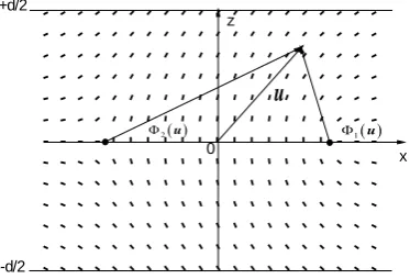
u  2 [12]. u is the distance between the origin

of coordinate and the observation point, Φ1

( )

u is the angle between the +1 2 singularity—observation point line and the x-axis, Φ2

( )

u is the angle between the −1 2 singularity—observation point line and the x-axis, as shown inFigure 1. θ is the angle between n and the x-axis. When the distance between the defects is re-laxed to r0 (any value wanted), liquid crystal cells with different cell gap are obtained using the plan-parallel technique.Take them as the initial conditions of our numerical calculations. The strong anchoring conditions on the bounding plates and free boundaries in the x-direction are used.

3. Results and Discussion

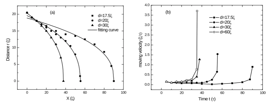
In order to analyze the influence of d on the behavior of the defect pair, the time dependence of the distance

r between the defect pair for different d with r0=20.5ξ and moving velocity of the defects as a function of time are shown inFigure 2.

The squares, circles and triangles represent numerical results with different cell gap d, respectively, and the full lines are the corresponding fitting curves with function of r

(

t0 t

)

α

∝ − [13] [21] inFigure2(a), where t0

is the coalescence time. α decreases andthe fitting error increases with the decrease of d, respectively. α decreases from 0.403 0.016± to 0.392±0.017 and the relative error increases from 3.9% to 4.3% when d

decreases from 30ξ to 20ξ . Further decrease d to 17.5ξ, α decreases to 0.387±0.052, the relative error is up to 13.4%, which means that the time dependence of r has deviated from the exponential law, as shown inFigure2(a).

u

( ) 1

Φ u

( )

2

Φ u

z +d/2

-d/2

[image:3.595.220.407.577.704.2]

x 0

(4)

[image:4.595.82.536.81.255.2]

Figure 2. (a) The time dependence of the distance r between the defect pair in a cell for different d with r₀=20.5ξ; (b)

Moving velocity of the defects as a function of time for different d with r₀=20.5ξ.

The distance between two isolated oppositely charged defects is described as r∝

(

t0−t

)

0.5 [13] [22]. In a confined geometry, the substrate anchoring forces influences the interactions between the defects. The thinner the cell gap, the greater the impact of the anchoring forces. Consequently, α decreases andthe fitting error in-creases with the decrease of d. When d decreases to 17.5ξ, the anchoring forces are so strong that they make the time dependence of r deviate from the exponential law.

The moving velocity of the defects increases rapidly with time because the elastic force between the two de-fects is F∝1r [12], but decreases with the decrease of d. It decreases slightly when d decreases from

60ξ to 30ξ, but rapidly when the cell gap decreases to 20ξ and 17.5ξ, as shown inFigure2(b). This re-sults in the increase of the coalescence time t0 with the decrease of d. The coalescence time slightly increas-es from 35.3τ to 37.75τ when d decreases from 60ξ to 30ξ, but soars to 55.5τ and 90τ when d decreases to 20ξ and 17.5ξ, respectively.

It indicates that the anchoring forces coming from the substrates produce a negligible effect on the defects when d≥30ξ . But, when d≤20ξ, the anchoring forces strongly affect the behavior of the dipole: inhibiting the moving movement of the defects. The thinner the cell gap, the greater the impact of the anchoring forces. Consequently, the moving velocity of the defects decreases with the decrease of the cell gap.

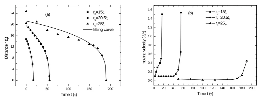
In order to analyze the influence of r0 on the behavior of the defect pair, the time dependence of the distance

r between the defect pair and moving velocity of the defects as a function of time for different r0 with 20

d= ξ are shown inFigure3.

α decreases with the increase of r0. It decreases from 0.441 0.033± to 0.392±0.017 when r0 increases from 15ξ to 20.5ξ . The time dependence of r follows the exponential law when r0≤20.5ξ . When r0 increases to 25ξ, α decreases to 0.300 ± 0.046, hence the relative error is up to 15%, which indicates the time dependence of r has deviated from the exponential law. The direct elastic interaction between the defects gives an elastic force F∝1r [12], resulting in the rapid decrease of the moving velocity with the increase of

r0, as shown inFigure3(b). Therefore, the coalescence time t 0 soars from 17τ to 190τ when r0 increases from 15ξ to 25ξ.

Increasing the initial distance has the same effect as reducing the cell gap: inhibiting the relative movement of the defects. The behavior of the pair depends on the competition between the attractive force, determined by the distance r between the defect pair, and the anchoring forces, determined by the cell gap d. The attractive force aggravates the annihilation process, while the anchoring forces inhibit the annihilation process. If the role of one kind of force is weakened, then the impact of the other will be relatively enhanced. Therefore, the impact of the anchoring forces are relatively enhanced with the increase of r0, which results in the decrease of α with the increase of r0 and the time dependence of r deviating from the exponential law when r0 increases to 25ξ. The anchoring forces and the attractive force must be balanced and the defects can be stable existence under certain conditions. In order to find the conditions, the dynamic behavior of the dipole is studied in detail by va-rying the cell gap d and the initial distance r0. The results are shown inFigure4 andFigure5.

0 20 40 60 80 100

0 5 10 15 20

D

is

tanc

e r

(

ξ

)

X (ξ)

d=17.5ξ d=20ξ d=30ξ fitting curve (a)

0 20 40 60 80 100

0.0 0.5 1.0 1.5 2.0 2.5 3.0 3.5 4.0

d=17.5ξ d=20ξ d=30ξ d=60ξ

m

ov

ing v

el

oc

ity

(

ξ/τ

)

(5)

[image:5.595.85.536.79.248.2]

Figure 3. (a) The time dependence of the distance r between the defect pair in a cell for different r0 with d = 20ξ. Squares,

circles and triangles represent numerical results. The full lines are the corresponding fitting curves with r

(

t0 t

)

α

∝ − ; (b) Moving velocity of the defects as a function of time for different r0 with d = 20ξ.

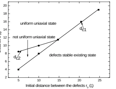
When r0 >15ξ, there are two equilibrium states, as shown in Figure4(a),Figure 4(b) andFigure5. The critical thicknesses dc1 are 19ξ and 16ξ, respectively. When d>dc1, the two defects annihilate because the attractive force between them plays a major role and a uniform uniaxial state is formed when the system is equilibrium. When d≤dc1, the defects can be stable existence because the anchoring forces are so strong that they can inhibit the relative movement of the defects. The thinner the cell gap, the greater the impact of the anc-horing forces. As a consequence, the relative moving distance decreases with the decrease of d.

When r0≤15ξ, there are three equilibrium states, divided by two critical thicknesses: dc1 and dc2, as shown inFigures4(c)-(e) andFigure5. The two critical thicknesses both change linearly with the initial dis-tance r0. The corresponding fitting equations are dc1=0.761r0 and dc2=6.95 0.31+ r0, respectively. When

1 c

d>d , the two defects annihilate. The annihilation process has delicate structures. When d >dc2, the two de-fects annihilate and a uniform uniaxial state is formed when the system is equilibrium. When dc2≥ >d dc1, the two defects annihilate. However, the system is not uniform uniaxial, but biaxial in the region where the defects collide. Since the two defects are oppositely charged and the total charge is conserved, the defects disappear when they collide. But, the director in the region where the defects collide distorts inhomogeneously, which creates the biaxial layers. The range of the cell gap d corresponding to this state increases with the decrease of

0

r . When d≤dc1, the dipole can be stable existence as the system is equilibrium because the anchoring forces play a major role under this condition.

4. Conclusions

The behavior of the dipole in a confined geometry depends on the competition between two kinds of forces: the attractive force and the anchoring force. The former aggravates the annihilation process, while the latter inhibits it. The system has three equilibrium states, divided by two critical thicknesses dc1 and dc2. When d>dc1, the pair annihilates, and the dynamics follows the function of r

(

t0 t

)

α

∝ − as d is sufficiently large. α decreases with the decrease of d or increase of r0. The annihilation process has delicate structures: when

0 15

r ≤ ξ and d>dc2 or r0>15ξ and d>dc1, the system is uniaxial at equilibrium state; while, when

0 15

r ≤ ξ and dc2≥ >d dc1, the system is biaxial in the region where the defects collide. When d≤dc1, the dipole can be stable existence.

As far as we know, it is the first time to discover the stable existence of the oppositely charged defects under certain conditions. This research plays a major role in the formation and control of topological defects, and has significant academic value for mediation of defects on colloidal particles in nematic liquid crystals.

Acknowledgements

We thank the Editor and the referee for their comments. Research of Z. Zhang is funded by National Natural

0 50 100 150 200

0 4 8 12 16 20 24

D

is

tanc

e r

(

ξ

)

Time t (τ)

r₀=15ξ r₀=20.5ξ r₀=25ξ fitting curve (a)

0 20 40 60 80 100 120 140 160 180 200 0.0

0.2 0.4 0.6 0.8 1.0 1.2 1.4 1.6

r₀=15ξ r₀=20.5ξ r₀=25ξ

m

ov

ing v

el

oc

ity

(

ξ

/

τ

)

(6)

[image:6.595.96.505.79.507.2]

Figure 4. The time dependence of β2

across the defect center parallel to the x-axis at equilibrium states: (a) r0=25ξ; (b) r0=20.5ξ; (c) r0=15ξ; (d) r0=10ξ; (e) r0=5ξ.

Figure 5. Phase diagram. The circles and squires represent numerical results of dc1 and dc2,

respec-tively; the full lines are the corresponding linear fits.

-20 -10 0 10 20

0.0 0.4 0.8

-20 -10 0 10 20

0.0 0.4 0.8

-20 -10 0 10 20

0.0 0.4 0.8

-20 -10 0 10 20

0.0 0.4 0.8

-20 -10 0 10 20

0.0 0.4 0.8

X (ξ) d=10ξ d=17.5ξ d=19ξ B ia xia lit y β 2 d=19.5ξ d=20ξ (a)

-20 -10 0 10 20

0.0 0.4 0.8

-20 -10 0 10 20

0.0 0.4 0.8

-20 -10 0 10 20

0.0 0.4 0.8

-20 -10 0 10 20

0.0 0.4 0.8

-20 -10 0 10 20

0.0 0.4 0.8

-20 -10 0 10 20

0.0 0.4 0.8

X (ξ) initial contion d=5ξ d=10ξ d=16ξ B ia xia lit y β 2 d=16.5ξ d=17ξ (b)

-15 -10 -5 0 5 10 15

0.0 0.4 0.8

-15 -10 -5 0 5 10 15

0.0 0.4 0.8

-15 -10 -5 0 5 10 15

0.0 0.4 0.8

-15 -10 -5 0 5 10 15

0.0 0.4 0.8

-15 -10 -5 0 5 10 15

0.0 0.4 0.8

X (ξ)

d=11ξ d=11.5ξ d=12ξ B ia xia lit y β 2 d=12.5ξ d=20ξ (c)

-10 -5 0 5 10

0.0 0.4 0.8

-10 -5 0 5 10

0.0 0.4 0.8

-10 -5 0 5 10

0.0 0.4 0.8

-10 -5 0 5 10

0.0 0.4 0.8

-10 -5 0 5 10

0.0 0.4 0.8

-10 -5 0 5 10

0.0 0.4 0.8

X (ξ)

d=5ξ d=8ξ d=8.5ξ d=9ξ B ia xia lit y β 2 d=9.5ξ d=10ξ (d)

-10 -5 0 5 10

0.0 0.4 0.8

-10 -5 0 5 10

0.0 0.4 0.8

-10 -5 0 5 10

0.0 0.4 0.8

-10 -5 0 5 10

0.0 0.4 0.8

-10 -5 0 5 10

0.0 0.4 0.8

-10 -5 0 5 10

0.0 0.4 0.8

-10 -5 0 5 10

0.0 0.4 0.8

X (ξ)

d=3ξ d=4.5ξ d=5ξ d=6ξ B ia xia lit y β

2 d=7ξ

d=8ξ

d=8.5ξ (e)

5 10 15 20 25

2 4 6 8 10 12 14 16 18 20 dc2

not uniform uniaxial state uniform uniaxial state

D

is

tanc

e d (

ξ

)

Initial distance between the defects r0 (ξ)

defects stable existing state

[image:6.595.222.416.546.694.2]

(7)

Science Foundation of China grant No. 11374087 and Key Subject Construction Project of Hebei Province University. This support is greatly appreciated.

References

[1] Carbone, G., Lombardo, G., Barberi, R., Musevic, I. and Tkalec, U. (2009) Physical Review Letters, 103, Article ID: 167801.

[2] Kurik, M.V. and Lavrentovich, O.D. (1988) Soviet Physics—Uspekhi, 31, 196-224.

http://iopscience.iop.org/0038-5670

http://dx.doi.org/10.1070/PU1988v031n03ABEH005710

[3] Tiribocchi, A., Gonnella, G., Marenduzzo, D. and Orlandini, E. (2010) Applied Physics Letters, 97, Article ID: 143505.

http://dx.doi.org/10.1063/1.3496472

[4] Takuya, O. and Jun-Ichi, F. (2012) Nature Communications, 3, 701-707. http://dx.doi.org/10.1038/ncomms1709

[5] Takuya, O., Jun-Ichi, F., Kosuke, S. and Yamaguchi, T. (2012) Physical Review E, 86, Article ID: 030701(R). [6] Tkalec, U., Ravnik, M., Čopar, S., Žumer, S. and Muševič, I. (2011) Science, 333, 62-65.

http://dx.doi.org/10.1126/science.1205705

[7] Ravnik, M., Alexander, G.P., Yeomans, J.M. and Žumer, S. (2011) Proceedings of the National Academy of Sciences

of the United States of America, 108, 5188-5192. http://dx.doi.org/10.1073/pnas.1015831108

[8] Fleury, J.B., Pires, D. and Galerne, Y. (2009) Physical Review Letters, 103, Article ID: 267801.

http://dx.doi.org/10.1103/PhysRevLett.103.267801

[9] Yoon, D.K., Choi, M.C., Kim, Y.H., Kim, M.W., Lavrentovich, O.D. and Jung, H.T. (2007) Nature Materials, 6, 866-870. http://dx.doi.org/10.1038/nmat2029

[10] Milette, J., Cowling, S.J., Toader, V., Lavigne, C., Saez, I.M., Lennox, R.B., Goodby, J.W. and Reven, L. (2012) Soft

Materials, 8, 173-179. http://dx.doi.org/10.1039/c1sm06604h

[11] Coursault, D., Grand, J., Zappone, B., Ayeb, H., Lévi, G., Félidj, N. and Lacaze, E. (2012) Advanced Materials, 24, 1461-1465. http://dx.doi.org/10.1002/adma.201103791

[12] Gennes, P.G. and Prost, J. (2008) The Physics of Liquid Crystals. 2nd Edition, Science Press, Beijing.

[13] Minoura, K., Kimura, Y., Ito, K., Hayakawa, R. and Miura, T. (1998) Physical Review E, 58, 643-649.

http://dx.doi.org/10.1103/PhysRevE.58.643

[14] Bogi, A., Martinot-Lagarde, P., Dozov, I. and Nobili, M. (2002) Physical Review Letters, 89, Article ID: 225501.

[15] Chuang, I., Turok, N. and Yurke, B. (1991) Physical Review Letters, 66, 2472-2475.

[16] Pargellis, A., Turok, N. and Yurke, B. (1991) Physical Review Letters, 67, 1570-1573.

[17] Chuang, I., Yurke, B., Pargellis, A.N. and Turok, N. (1993) Physical Review E, 47, 3343-3356.

[18] Pargellis, A.N., Mendez, J., Srinivasarao, M. and Yurke, B. (1996) Physical Review E, 53, R25-R28.

http://dx.doi.org/10.1103/PhysRevE.53.R25

[19] Minoura, K., Kimura, Y., Ito, K. and Hayakawa, R. (1997) Molecular Crystals and Liquid Crystals Science and

Tech-nology. Section A: Molecular Crystals and Liquid Crystals, 302, 345-355.

http://dx.doi.org/10.1080/10587259708041847

[20] Wang, W., Shiwaku, T. and Hashimoto, T. (1998) The Journal of Chemical Physics, 108, 1618-1625.

http://dx.doi.org/10.1063/1.475532

[21] Svensek, D. and Žumer, S. (2002) Physical Review E, 66, Article ID: 021712.

[22] Tóth, G., Denniston, C. and Yeomans, J.M. (2002) Physical Review Letters, 88, Article ID: 105504.

[23] Bradač, Z., Kralj, S., Svetec, M. and Žumer, S. (2003) Physical Review E, 67, Article ID: 050702. [24] Svetec, M., Kralj, S., Bradac, Z. and Žumer, S. (2006) The European Physical Journal E, 20, 71-79.

http://dx.doi.org/10.1140/epje/i2005-10120-9

(8)

[26] Giomi, L., Bowick, M.J., Ma, X. and Marchetti, M.C. (2013) Physical Review Letters, 110, Article ID: 228101.

[27] Peroli, G.G. and Virga, E.G. (1999) Physical Review E, 59, 3027-3032. http://dx.doi.org/10.1103/PhysRevE.59.3027

[28] Lu, L.X. and Zhang, Z.D. Chinese Physics B, in Press.

[29] Bisi, F., Gartland, E.C., Rosso, R. and Virga, E.G. (2003) Physical Review E, 68, Article ID: 021707.

[30] Barberi, R., Ciuchi, F., Durand, G., Iovane, M., Sikharulidze, D., Sonnet, A. and Virga, E. (2004) The European

Phys-ical Journal E: Soft Matter, 13, 61-71. http://dx.doi.org/10.1140/epje/e2004-00040-5

[31] Lombardo, G., Ayeb, H. and Barberi, R. (2008) Physical Review E, 77, Article ID: 051708. [32] Schopohl, N. and Sluckin, T.J. (1987) Physical Review Letters, 59, 2582-2584.

[33] Lu, L.X., Zhang, Z.D. and Zhou, X. (2013) Acta Physica Sinica, 62, Article ID: 226101. [34] Zhou, X. and Zhang, Z.D. (2013) International Journal of Molecular Sciences, 14, 24135-24153.

http://dx.doi.org/10.3390/ijms141224135

(9)

Appendix

The free-energy density f of a NLC without external fieldcan be expressed as

e b

f = f + f . (A1)

They are, respectively, the elastic and the bulk free-energy densities. The former is induced by the inhomo-geneous order in LCs. It can be given the form

1 2 3

ij ij ij ik ij ik

e

k k j k k j

Q Q Q Q Q Q

f L L L

x x x x x x

∂ ∂ ∂ ∂ ∂ ∂

= + +

∂ ∂ ∂ ∂ ∂ ∂ , (A2)

where L L1, 2 and L3 are elastic constants. The latter is a potential that depends on Q. It is conventionally described by an expansion in Q up to the fourth order

( )

2

2 3 2

b

f = AtrQ + BtrQ +C trQ . (A3)

Usually it is assumed that A A T0

(

T

)

∗

= − , where T is temperature and T∗ is the supercooling tempera-ture. A0, B and C are coefficients. The traceless and symmetry of Q are taken into account by the intro-duction of the Lagrange parameter tensor [32]: Λ =ij λ δ0 ij−ε λijk k. The full free-energy functional is

(

,

)

_e 2

(

)

_b

f Q Λ = f + tr ΛQ + f . (A4) The calculation can be simplified by dimensionless variables. Here, we follow the rescaling of Schopohl and Sluckin [32] by defining the following dimensionless quantities