Deep Cutting Plane Inequalities for Stochastic Non Preemptive Single Machine Scheduling Problem

(1)

http://dx.doi.org/10.4236/ajor.2015.52006

Deep Cutting Plane Inequalities for

Stochastic Non-Preemptive Single

Machine Scheduling Problem

Fei Yang, Shengyuan Chen

Department of Mathematics and Statistics, York University, Toronto, Canada Email: yangfei0743@hotmail.com, chensy@mathstat.yorku.ca

Received 13 February 2015; accepted 1 March 2015; published 4 March 2015

This work is licensed under the Creative Commons Attribution International License (CC BY). http://creativecommons.org/licenses/by/4.0/

Abstract

We study the classical single machine scheduling problem but with uncertainty. A robust optimi-zation model is presented, and an effective deep cut is derived. Numerical experiments show ef-fectiveness of the derived cut.

Keywords

Single Machine Scheduling, Cut Generation, Robust Optimization

1. Introduction

The problem of scheduling a single machine to minimize the total weighted completion time is one of most well-studied problems in the area of scheduling theory in [1] [2]. The textbook by Leung [3] provided excel-lence coverage of most advantage topic in scheduling problem. In this paper, we will concentrate on the situa-tion that the period of length of each job is uncertain; addisitua-tionally, only a set of possible period of length scena-rios are predictable. Traditional, two classic approaches are used to manage this problem: Stochastic Program-ming and Robust Optimization. The Stochastic ProgramProgram-ming approach optimizes the expected value of total weighted completion time over all scenarios. However, since the accurate probability of each scenario usually is difficult to achieve [4] [5], the Worst Case Scenario Analysis in Robust Optimization should be a better choice to manage this problem [6].

(2)

Zhao’s paper [10]; in Section 3, we will deeply explain the worst case scenario analysis and provide numerical example. In the Section 4, we run the computational test and display the methodology of efficient cutting in-equalities selection for this model; finally, our extensive computational results are reported to demonstrate the efficiency and effectiveness of the proposed solution procedures.

The most common assumptions for non-preemptive single machine scheduling problem are shown in the fol-lowing section. A set of n jobs are required to be executed in a single machine, and each job demands a period of processing length L. The machine can only execute one job at a time.

Variable Definition:

• s n, are positive integers.

• S =

{

1,,s

}

the set of scenarios.

• N=

{

1,,n

}

the set of jobs required to be executed.

• W_j = the cost per unit of job j in the system.

• s j

L = the period of processing length of job j in scenario s.

• s j

C = the completion time of job j in scenario s.

• δ =ij 1 means the jobs i precedes job j in the schedule, and δ =ij 0 otherwise.

We consider the scheduling problem in the single machine environment without preemptive jobs. The purpose is to minimize the expected total weighted completion time over all scenarios. The stochastic model is shown in following.

min z (1)

. . _j s_j

j N

s t z W C s S

∈

≥

∑

∀ ∈ (2)

,

s s s j j j ij

i N j

C L Lδ s S j N

∈ −

≥ +

_∑

∀ ∈ ∈ (3)

1 , ,

ij ji i j N i j

δ +δ = ∀ ∈ ≠ (4)

1 , , , , ,

ij jk ik i j k N i j i k k j

δ +δ −δ ≤ ∀ ∈ ≠ ≠ ≠ (5)

{ }

0,1 , ,

ij i j N i j

δ ∈ ∀ ∈ ≠ (6)

where

• Constraint (1) ensures that the optimal value is the minimum total weighted completion time in worst case scenarios;

• Constraint (2) means the completion time of job j in scenario s should be greater or equal than the processing length of job j in scenario s plus the total completion time of the jobs which are executed to start before job i

in scenario s. It ensures that no job is scheduled to start while another job is being executed;

• Constraint (3) ensures that a job can be only executed once in the system;

• Constraint (4) enforce δ =ik 1 when δij =δjk =1;

• Constraint (5) declares that δij is a binary number.

The model is an NP-hard problem as shown in [11]. Although time-indexed linear programming formulations have received a great attention in solving single machine scheduling problem, see [12], the NP-hard scheduling problem is one of the most difficult questions. One possible solution is to generate cutting plane inequalities, as shown in [9] [13] [14], for machine scheduling problem. In the next section, we will develop a large set of in-equalities that valid for this model.

2. A Set of Cutting Plane Inequalities for

L

In this section, I will introduce a large set of inequalities which are valid for L, and a sufficient condition that is necessary to estimate those inequalities. In order to find those cutting inequalities, we divide the set of jobs n

into three parts: {x}, I and N−

{

{ }

x I

}

, where x is an individual job, I is a nonempty subset of N. Let p be a permutation of I, and , ,

k x p

s s ∈ ∀ ∈S k I. Suppose that i< ∀j, i j, ∈I. If

1 1

pk x pk x

i j j i

I I

s s s s

p p p p

k k

L L L L

= =

≥

(3)

then

( )

1 1

p

p k x

x t t t I I s s s s

x x p p

t k

Q C L C L C G L

= =

 

= _ + _≥

 

∑

(8)

is valid for L where

( )

1 1 1 1

( .

p

p k x

x t x

t v

I I I t

s

s s

x x p p x

t t k v

G L L L L L L

= = = =

 

= + _ + _

 

∑

∑∑

∑

(9)

Proof. We assume that

( )

₁

(

x pt ₁ pk x

)

t t s s

I s I s

x x p p

t k

Q C =

∑

₌ L C +

∑

₌ L C . Let C be a feasible schedule, and Q C

( )

be the minimum value of Q C

( )

over all C. Our purpose is to find Q C

( )

. Three steps are required in order to reach the goal:

a) Determine that any jobs in N−

{

xI

}

should be scheduled to start after all jobs in

{

xI

}

in Q C

( )

. b) Determine that Q C

( )

is unchanged or holding one condition if we switch the scheduling order of job x

and any job in I.

c) Determine that Q C

( )

is unchanged or holding the same condition as in b) if we switch the order of any two jobs in I.

If all three steps are satisfied, the schedule of all jobs in

{

xI

}

is settled and we get Q C

( )

. I will show how each step works in the following:

[Step 1] If any job in N−

{

xI

}

is scheduled to start before all jobs in

{

xI

}

, Q C

( )

will increase be-cause it will rise the value of spt

x

C or x

t

s p

C . Therefore, it is reasonable that jobs in N−

{

xI

}

{

xI

}

in Q C

( )

. Also, the schedule of all jobs in

{

xI

}

should be tight in all scenarios for the same reason.

[Step 2] Assume that job x follows job pi in schedule immediately, where pi∈I. Let C be the

comple-tion time resulting from switching the order of job x and pi while keeping the same completion time for all

other jobs, we can get:

{

}

if , ;

if , , .

i

a a x p

a a a

b p x i

a

b i

C L b x a S

C C L b p a S

C b N x p a S

 − = ∈  =_ + = ∈  = − ∈  Then,

( )

(

)

(

)

( )

1

1 1 1 1 1 1

1

1 1 1 1 1 1

.

p p p p

p t k x k x k x

x t x

i t t i i t t

p p p

p k x k k x

x t x

t t i t t

I i I I I I

s s s s

s s

x x p p p p p x p p

t t k k t i k

I i I I I I

s s s

s s

x x p p p x p p

t t k k t i k

Q C L C L L C L C L L C

L C L C L C L C Q C

− = = = = = + = − = = = = = + = = − + + + + = + + + =

∑

∑∑

∑

∑ ∑

∑

∑∑

∑

∑ ∑

The same result holds if pi follows x immediately in C, so we can conclude that it makes no difference

when we switch the order of job x and any job in I. on the other hand, it indicates Q C

( )

is the same when job

x is scheduled to start before all jobs in I, after any one job in I, after any two jobs in I,⋅⋅⋅,fter all jobs in I. In addition to that, in Step 1, we known that all jobs in N−

{

xI

}

{

xI

}

, thus we can conclude that all jobs are scheduled in the order:{x}, all jobs in I, and jobs inN−

{

xI

}

.

[Step 3] Suppose that job pj is scheduled to start after job pi in C, where i< j and p pi, j∈I. Let C

be the completion time resulting from switching the order of pi and pj, while keeping the same completion

for all other jobs. We have:

{

}

if , ;

if , , .

i j

j i

a a

p p i

a a a

b p p j

a

b i j

C L b p a S

C C L b p a S

C b N p p a S

(4)

Then,

( )

(

)

(

)

( )

1

1 1 1 1

1 1 1

1 1

.

p p

p k x k x x

x t

t t i i j

pk x x pk x

j j i t t

pk x pk x

i j j i

I i I I

s s

s s s s

s

x x p p p p p

t t k k

I I I

s s s s s

p p p p p

k t j k

I I

s s s s

p p p p

k k

Q C L C L C L C L

L C L L C

Q C L L L L

− = = = = = = + = = = = + + + + − + = + −

∑

∑∑

∑

∑ ∑

∑

Therefore, Q C

( )

≥Q C

( )

if ₁ pk x ₁ pk x

i j j i

s s

I s I s

p p p p k= L L ≥ k= L L

∑

. It proved that, with this condition, the jobs in I should be scheduled in order p p1, 2,,pI in Q C

( )

.

In a sum of step 1, 2 and 3, we can conclude that the minimum value of Q(C) can be achieved if the jobs are settled in the order: x p p, 1, 2,,pI , and jobs in N−

{

xI

}

with condition (7). We can write the inequality

as

(

)

(

)

1 1 1 1 1 1 .

p p

p k x p k x

x t x t x

t t t v

s s

I s I s I s I I t s s

x x p p x x p p x

t= L C + k= L C ≥ t= L L + t= k= L v= L +L

∑

∑ ∑

∑

Specific Cases. Instead of adding all inequalities to the model, we focus on three special cases which can be

generated efficiently.

First, assume that 1, ,

k

x p

I = s =u s =s, and then we found that condition (7) has always held. Thus, (8) be-comes

.

u s s u u s s u s u x x t t x x t t t x

L C +L C ≥L L +L L +L L (10)

The numbers of inequalities are 2

2 2

s n

        .

Second, suppose that ₁ ₂ ₃

I

p p p p

s =s =s ==s and I = −n 1, so the condition equivalent to

j i i j u u p p s s p p L L

L ≤ L (11)

with i< j,∀i j, ∈I. Suppose we sort Lup_i Lsp_i in a non-decreasing order, then we have

1 2

I

u u u

p p p

s s s

p p p

L L L

L ≤ L ≤≤ L (12)

the inequality becomes to

1 1 1

.

t t t v

I I t

u s s u u s s u u

x x p p x x p p x

t t v

L C L C L L L L L

= = =

+ ≥ + _ + _

 

∑

(13)

In total, we can generate

(

)

2 1

2

s

n s s n

 

= −  

 

inequalities.

Third, suppose there are N jobs and N scenarios,

1 2 3 I

p p p p

s ≠s ≠s ≠≠s and I= −n 1, then the condition can be rewritten as

1 1

.

N N

t u t u e e k k

t t

L L L L

= =

≥

(5)

Then the inequality becomes

1 1 1

1 1 1 1

.

t t t

t t v

I

N N

u k u k u u

x x x p p p

k t k

I

N N t

u k u k u u u

x x x p p p x

k t k v

L C C L C C

L L L L L L L

= = =

= = = =

   

− + −

   

   

   

≥ _ − _+ _ − _ +   

 

 

 



∑

∑ ∑

∑

∑ ∑

∑

(15)

We can totally generate n2 inequalities in this case.

Example. Let L11=3,L12 =5,L13=7,L12=6,L22=4,L32=5,L31=4,L32=7, and 4L33= , the following inequali-ties are valid for this model:

1 2

2 1

4C +3C ≥50 (16)

1 3 3

2 1 3

7C +3C +7C ≥157 (17)

1 1 2

1 3 2

6C +5C +5C ≥143. (18) In inequality (16), x=2,I=

{ }

1 and s1 =2,s2 =1. In inequality (17), x=2,I =

{ }

1, 3 ;p1=1,p2=3 and

1 3 1, 2 3

s =s = s = . In inequality (18), x=2,I=

{ }

1, 3 ;p1=1,p2=3 and s1 =s3 =2,s2 =1. Clearly, (16) is an example of special case one, and (17); (18) are examples of special case two.

3. Worst-Case Scenario Analyses

In stochastic programming [4], it is assumed that we have recognized the probability distribution of the data set, and the goal is to minimize the expected value over all scenarios. On the other hand, worst case scenario analy-sis can be considered as another method to solve the stochastic model, its goal is to find a solution that minimize the cost in worst case scenario [6]. Worst-case design is not intended to necessarily replace expected value op-timization when the underlying uncertainty is stochastic. However, wise decision making requires the justifica-tion of policies based on expected value optimizajustifica-tion in view of the worst-case scenario. Optimality does not depend on any single scenario but on all the scenarios under consideration. Worst-case optimal decisions pro-vide guaranteed optimal performance for systems operating within the specified scenario range indicating the uncertainty. Here is a simple example to give us the real solution of worst case scenario method.

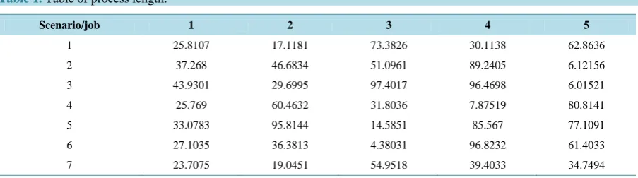
Example. We randomly generated a data set including 5 jobs and 7 scenarios in the Table 1, and assume all

the coefficients of completion time be 1, so how to scheduling this single machine scheduling problem in worst case scenario model?

After solving this problem, we got the following result: the optimal solution is 783.1717, and the scheduling order is 1→ → → →3 5 2 4. Additionally, since our objective function is to minimize the cost in worst case scenario, the relationship of optimal cost between worst case scenario and each single scenario should be inter-esting. Thus, we calculated the minimum cost and the optimal order across each scenario separately, and then we can get the optimal cost of other scenarios by this order. For instance, the optimal order for scenario 1 is

[image:5.595.88.540.596.722.2]

2→ → → →1 4 5 3 and optimal value is 478.28, so the cost will be 713.55 in scenario 2 and 723.06 in scenario 3 if we use this order. The result is displayed in Table 2.

Table 1. Table of process length.

Scenario/job 1 2 3 4 5

1 25.8107 17.1181 73.3826 30.1138 62.8636

2 37.268 46.6834 51.0961 89.2405 6.12156

3 43.9301 29.6995 97.4017 96.4698 6.01521

4 25.769 60.4632 31.8036 7.87519 80.8141

5 33.0783 95.8144 14.5851 85.567 77.1091

6 27.1035 36.3813 4.38031 96.8232 61.4033

(6)

[image:6.595.91.534.391.446.2]

Table 2.Table of worst case scenario analysis.

Scenario Optimalorder\optimal value z1 z2 z3 z4 z5 z6 z7 Max

Worst case 675.52 591.7 783.17 627.3 732.26 506.83 520.09 783.17

1 1→ → → →3 5 2 4 478.28 713.55 723.06 622.45 1,036.89 707.98 432.72 1,036.89 2 2→ → → →1 4 5 3 645.79 511.16 586.17 760.02 920.04 630.16 475.02 920.04 3 5→ → → →1 4 5 3 593.83 558.72 571.01 770.78 1,053.76 731.88 454.81 1,053.76 4 4→ → → →1 3 2 5 571.06 848.05 1,015.69 439.6 872.64 739.84 529.54 1,015.69 5 3→ → → →1 5 4 2 736.09 648.08 903.41 580.75 703.51 544.55 571.69 903.41 6 3→ → → →1 2 5 4 677.35 646.09 860.33 612.99 732.47 459.09 535.63 860.33 7 2→ → → →1 5 4 3 511.03 630.43 632.6 695.39 1,028.43 672.56 428.06 1,028.43

To be surprised, the optimal order in worst case scenario model is following none of those scenarios. Also, the optimal cost in worst case scenario model is less than the largest cost in each scenario. To explain more specifi-cally, if we choose to operate the machine by the optimal order of anyone one of scenario, the cost in worst situa-tion is larger than the cost made from operating the machine by the optimal order from worst case scenario model.

4. Computational Results

In this section, we will show all the results from our computational test. Since we have already proved that our inequalities are working for this single machine scheduling problem, in order to test the efficiency of our inequi-ties, we compare the computational time from solving the original model without any inequalities added, with all inequalities and with limited number of inequalities. We manage the model in following procedure:

Model

Solving LP Without Inequalities

Solving IP Without Inequalities

Solving LP With all Inequalities

Solving IP With Limited

Inequalities

Our computational test indicated that adding all inequalities would increase computational time because of the time to generate those inequalities. In fact, many of those inequalities actually cut nothing in feasible region. In order to save computational time, we should select the most valuable inequalities to the model instead of adding all the inequalities.

It is interesting that the slack values of some inequalities are zero in the integer model. It is a message that those inequalities go through the optimal point. On the other side, it means that the inequalities we generate are efficient. Thus, our inequalities are helpful to reduce the computational time if we add the right equalities. The idea is that we add top n equalities with smallest slack value selecting from the case one and case two. In the test, we found that the slack value of inequalities from case two was larger than the slack value in case one.

Thus, the inequalities we add in the model are the top N smallest slack value inequalities from case one. We randomly generated 45 examples of the model with size range from n = 50 and s = 5 to n = 110 and s = 10. The number of variables and constraints, totally, ranged between 2710 variables and 120,305 constraints to 13,091 variables to 1,308,020 constraints. Note that most of constraints are the triangle constraints; hence it will be bet-ter to take the possible advantage from selecting the essential triangle constraints rather than adding all of them in the formulation.

The coefficients of decision variable in objective function, w w1, 2,,wn were randomly generated from a

(7)

[image:7.595.90.536.137.724.2]

We summarized the computational results in Table 3 where the column “Reduction” indicated the reduction in percentage of the integer model without cut.

Table 3. Computational result.

Test LP without cut IP without cut IP with cut Reduction

# M N Solution Time Solution Time Solution Time Time

1 5 50 285,190.90 46.502 285,223.90 28.095 285,223.90 9.819 65.1%

2 5 50 236,067.76 31.654 236,090.70 34.922 236,090.70 8.014 77.1%

3 5 50 237,015.60 22.901 237,044.73 8.57 237,044.73 7.757 9.5%

4 5 50 275,593.68 55.268 275,628.03 21.237 275,628.03 11.449 46.1%

5 5 55 361,997.38 52.182 362,023.25 17.628 362,023.25 13.198 25.1%

6 5 55 261,649.06 29.094 261,649.25 18.299 261,649.25 10.437 43.0%

7 5 55 270,083.84 49.187 270,107.37 26.184 270,107.37 15.643 40.3%

8 5 60 397,399.62 116.099 397,434.55 31.048 397,434.55 17.506 43.6%

9 5 60 323,017.61 91 323,046.88 16.291 3,230,468.88 18.175 −11.6%

10 5 60 404,668.08 104.334 404,710.25 29.914 404,710.25 17.262 42.3%

11 5 60 363,027.82 178.153 363,058.15 20.321 363,058.15 16.51 18.8%

12 5 60 349,591.46 126.799 349,611.41 19.02 3,496,119.41 17.718 6.9%

13 5 65 382,837.06 213.886 383,860.97 34.578 383,860.97 28.003 19.0%

14 5 65 413,995.33 211.687 414,032.29 44.976 414,032.29 29.317 34.8%

15 5 65 382,166.31 252.163 382,198.07 31.689 382,198.07 29.532 6.8%

16 5 70 411,558.15 254.626 411,586.33 98.236 411,586.33 27.901 71.6%

17 5 70 469,010.64 161.522 469,047.28 45.364 469,047.28 20.717 54.3%

18 5 70 417,065.63 214.37 417,108.05 58.647 417,108.05 24.18 58.8%

19 5 75 584,177.79 510.956 584,233.83 64.348 584,233.83 44.325 31.1%

20 5 75 540,849.16 290.956 540,875.83 63.563 540,875.83 73.82 −16.1%

21 5 75 562,198.21 488.701 562,254.84 58.734 562,254.84 41.527 29.3%

22 6 80 668,924.38 629.462 668,988.32 73.243 668,988.32 48.493 33.8%

23 6 80 619,362.39 612.39 619,415.30 76.192 619,415.30 51.372 32.6%

24 6 80 677,651.25 527.482 677,692.17 57.38 677,692.17 42.183 26.5%

25 6 85 650,652.28 1935.93 650,715.63 105.097 650,715.63 58.228 44.6%

26 6 85 772,202.64 529.433 772,253.72 72.39 772,253.72 30.233 58.2%

27 6 85 758,265.28 2837.245 758,301.32 94.422 758,301.32 83.143 12.0%

28 6 90 825,903.26 3015.75 825,959.83 85.276 825,959.83 85.76 −0.6%

29 6 90 877,343.92 989.38 877,411.27 64.829 877,411.27 76.249 −17.6%

30 6 90 902,635.94 2102.47 902,689.38 186.093 902,689.38 123.257 33.8%

31 6 95 946,268.86 3604.92 946,304.24 146.63 946,304.24 98.38 32.9%

32 6 95 891,488.27 2585.86 891,536.28 139.62 891,536.28 108.284 22.4%

33 6 95 792,987.93 2719.35 793,026.32 87.32 793,026.32 85.18 2.5%

34 6 100 996,203.26 4952.72 996,560.26 156.28 996,560.26 110.106 29.6%

(8)

Computational time is decreased for 85% of tests with our equalities added. On average, the reduction is about 28.6%.

References

[1] Hall, L., Shmoys, B., Wein, J. and Schulz, A. (1997) Scheduling to Minimize Average Completion Time: Off-Line and On-Line Approximation Algorithms. Mathematics of Operation Research, 22, 513-544.

http://dx.doi.org/10.1287/moor.22.3.513

[2] Yang, J. and Yu, G. (2002) On the Robust Single Machine Scheduling Problem. Journal of Combinational Optimiza-tion, 6, 17-33. http://dx.doi.org/10.1023/A:1013333232691

[3] Leung, J.Y.-T. (2004) Handbook of Scheduling: Algorithms, Models, and Performance Analysis. Chapman & Hall/ CRC, US.

[4] Birge, J.R. and Franois, L. (1997) Introduction to Stochastic Programming. Springer, Berlin.

[5] Mastrolilli, M., Mutsanas, N. and Svensson, O. (2008) Approximating Single Machine Scheduling with Scenarios.

Computer Science, 5171, 153-164.

[6] Rustem, B. and Howe, M. (2002) Algorithms for Worst-Case Design and Applications to Risk Management. The Princeton University Press, Princeton.

[7] Hamada, T. and Glazebrook, K.D. (1993) A Bayesian Sequential Single Machine Scheduling Problem to Minimize the Expected Weighted Sum of Flow Times of Jobs with Exponential Processing Times. Operation Research, 41, 924-934. http://dx.doi.org/10.1287/opre.41.5.924

[8] Nemhauser, G.L. and Wolsey, L.A. (1988) Integer and Combinatorial Optimization. Wiley, New York. http://dx.doi.org/10.1002/9781118627372

[9] Soric, K. (2000) A Cutting Plane Algorithm for a Single Machine Scheduling Problems. European Journal of Opera-tional Research, 127, 383-393. http://dx.doi.org/10.1016/S0377-2217(99)00493-2

[10] de Farias Jr., I.R., Zhao, H. and Zhao, M. (2010) A Family of Inequalities Valid for the Robust Single Machine Sche-duling Polyhedron. Computers & Operations Research, 37, 1610-1614. http://dx.doi.org/10.1016/j.cor.2009.12.001 [11] Garey, M.R. and Johnson, D.S. (1979) Computers and Intractability: A Guide to the Theory of np-Completeness.

Freeman.

[12] de Sousa, J.P. and Wolsey, L.A. (1992) A Time-Indexed Formulation of Non-Preemptive Single-Machine Scheduling Problems. Mathematical Programming, 54, 353-367. http://dx.doi.org/10.1007/BF01586059

[13] Queyranne, M. (1993) Structure of a Simple Scheduling Polyhedron. Mathematical Pragramming, 58, 263-285. http://dx.doi.org/10.1007/BF01581271