http://dx.doi.org/10.4236/jmp.2015.63029
Accelerating Expansion in a Closed Universe
Martin Tamm
Department of Mathematics, University of Stockholm, Stockholm, Sweden Email: matamm@math.su.se
Received 9 October 2014; accepted 16 February 2015; published 25 February 2015
Copyright © 2015 by author and Scientific Research Publishing Inc.
This work is licensed under the Creative Commons Attribution International License (CC BY).
http://creativecommons.org/licenses/by/4.0/
Abstract
In this paper, I suggest a possible explanation for the accelerating expansion of the universe. This model does not require any dark energy or quintessence. Rather, the idea is to suggest a different view on the origin of general relativity. Since it is very difficult to say something in general, I will mainly restrict myself to the case of very low curvature. The question about the underlying rea-sons for the acceleration is also closely related to the question whether the universe is a finite or infinite. It is part of the purpose of this paper to argue that a phase of accelerating expansion may be very well compatible with the idea of a closed universe.
Keywords
Dark Energy Theory, Quintessence, Modified Gravity, General Relativity, Accelerating Expansion, Cosmological Constant
1. Is the Universe Closed or Open?
The question whether the universe has a finite or infinite extension in space and time is a long open problem. Already when the 16th century philosopher Giordano Bruno claimed the universe to be infinite, the question was highly controversial. However, it is only after the birth of general relativity that it has become a scientific one instead of just a philosophical one.
It can very well be questioned whether it will ever be possible to actually prove that our universe is closed or open. What we can do is to compare different models for cosmology and try to see which one of them is in best agreement with observations. And in the same time apply Ockham’s razor to avoid building theories on more uncertain assumptions then necessary.
conclusion is that the repulsive effect will become stronger and stronger, hence leaving little room for closed models. Many different related scenarios have been discussed, see for example [4] [5].
However, it has turned out to be difficult to explain the origin and properties of this dark energy or quintes-sence. The most reliable information that we have about it comes from supernova redshifts (see [6]). Other at-tempts to explain the accelerating expansion have started from the idea that it is perhaps general relativity which is incomplete (see for instance [7]). On the other hand, it is not easy to introduce new elements into this re-markable theory without spoiling its natural simplicity.
In this paper, I will take the point of view that a phase of accelerating expansion can be a very natural pheno-menon in a closed universe, and that no dark energy or quintessence is necessary to explain it. The method of approach will be to try to analyze the origin of general relativity in the limit of very small curvature. In addition, I will assume that the total four-volume of the universe, from the Big Bang to the Big Crunch, is fixed. This idea is very natural if we give up the view that space-time is an empty arena for particles, but rather consider it to be an active part of the world which is also built out of some (finite number of) constituents. On the other hand, it should in the same time be noted that this kind of condition does not make sense if we want to explain the acce-leration in open universes. Thus finiteness is really an essential condition.
Before we go further, let me state explicitly that for all phenomena on a normal astronomical scale (perhaps also excluding situations where the curvature is extremely high), I still consider usual general relativity to be more or less a perfect theory: every theory which claims to be realistic must in the end reduce to it on such a scale, and I will in fact also use ordinary general relativity to motivate some of the results in this paper. Never-theless, in cosmology there have for a long time been indications that Einstein’s original equations may not be the last word.
The mathematical methods of this paper are rather unsophisticated. A deeper understanding can presumably be reached with methods from, in particular, optimization and control theory. But this is so far a project for the future. In this paper, I have restricted myself to just trying to show what kind of phenomena can occur.
Most of the following computations have been carried out using Mathematica. The author is indebted to the book by Parker & Christensen (see [8]) for the basic method to compute curvature with a computer.
Many physicists believe that the final answer to the question about dark energy should come from micro- physics, and this may very well be so. There is however presently no agreement about what such as answer would look like. Therefor, it may be that general relativity still has something to contribute.
2. Classical Relativistic Cosmology
One of the historically most influential models for cosmology is the closed Friedmann model (see [9]). Let us consider a compact, homogeneous, isotropic universe with the following metric in spacial, spherical coordinates
, ,
χ θ ϕ:
( )
2(
(
)
)
2 2 2 2 2 2 2
ds = −dt +a t dχ +sin χ θd +sinθ ϕd (1)
Since we will mainly be dealing with closed models, the function a t
( )
can naturally be thought of as the ra-dius of the universe at time t as well as in terms of the nowadays more common scale factor.The field equations of general relativity are given by
8π
ij ij
G = T (2)
where Gij is the Einstein tensor and Tij is the stress-energy tensor (see further e.g. [10] [11]). The most useful
component of (2) in cosmology is the time-time component which reads
( )
( )
( )
( )
2
0
2 2 3
6
6 a 6 a
t t
a t a t a t
∂
+ =
∂
(3)
where a0 is a positive constant which is usually considered to represent some kind of total mass of the universe. After simplifications we get
( )
2( )
0 1a a
t
t a t
∂
= −
∂
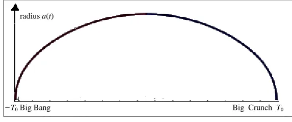
It is easy to see that the positive solution to this equation, starting from the value 0 at the Big Bang, will grow up to its maximal value a0 and after that decrease in a symmetric way down to zero at the Big Crunch. In fact, the solution to (4) is a cycloidal function as depicted in Figure 1. It can be noted that this model gives a closed universe no matter how large or small the mass a0 is.
The closed Friedmann model is nowadays neither the best nor the most popular model for cosmology. Never-theless, it may serve as a natural comparison with the model in this paper.
3. What Is the Origin of the Field Equations?
Simplifying somewhat, one can say that Einstein’s original way of motivating the field equations of general re-lativity was that, assuming the equivalence of all possible frames of reference and adding a few very natural as-sumptions, these are the only possible ones. The only one of these additional assumptions which did not appear to be absolutely indispensable was the idea that space-time in the absence of mass-energy should be flat. Aban-doning this assumption opened up for a non-zero cosmological constant. Ever since Einstein reluctantly admit-ted this constant into his equations (see [12]), it has lived a life of its own: it has appeared in cosmological theo-ries as well as in fundamental theotheo-ries in various shapes, and with the discovery of the accelerating expansion of the universe it seems to have become something which we will have to learn to live with.
Is this bad news for general relativity? The answer to this question of course depends on our perspective: if we cannot find a good motivation for the cosmological constant or other modifications, then some of the natural simplicity of the theory is actually lost. On the other hand, searching for such a motivation could give us clues to an even more natural theory.
In a universe with accelerating expansion there may also be other problems with the field equations. One of the things Einstein was not prepared to give up was the conservation law for mass-energy. This is also built into the field equations in the disguise of the Bianchi identities. But in our universe, potential energy seems to be ra-pidly growing (because galaxies are drifting apart). In the same time photons are loosing energy (because of the red-shift). It is true that the conservation law which is implied by the Bianchi identities is not entirely equivalent to what we usually mean by energy conservation (see [13]). It is also true that the idea of potential energy does not fit into general relativity and that conservation of gravitational energy usually is considered only in the con-text of asymptotic flatness or other additional assumptions. It may be a little bit too hasty to give up mass-energy conservation altogether. Nevertheless, it should definitely be kept in mind that even if there is a fundamental conservation law, we do not really yet know what it is that is conserved. In that case, it is also not certain that the Bianchi identities, and hence the traditional field equations, the Robertson-Walker metric etc. really make sense in the context of global cosmology. One possible perspective on this issue is to say that the problem with mass-energy conservation in general relativity is a consequence of the fact that we are trying to make a three- dimensional conservation law out of something which is intrinsically four-dimensional. This way of thinking is also part of the motivation for Principle 1 below.
A traditional way of deriving the field equations is by means of the Hilbert-Palatini variational principle, which is the standard formulation of the Principle of Least Action in general relativity:
d 0
R V
δ
∫
= (5)The Principle of Least Action in turn has a long history and is usually considered to be due to Maupertius [14],
Big Crunch T0
−T0 Big Bang
[image:3.595.167.454.590.710.2]radius a(t)
although historically he may not have been the first one to formulate it. In Maupertius’ interpretation, this prin-ciple expresses the ultimate economy of nature, in the sense that nature always develops in the way which de-mands the least effort. However, already Euler observed that the developments which occur do not always mi-nimize the action globally, and nowadays the Principle of Least Action is generally only considered to be a technical way of deriving the field equations, without any philosophical implications what so ever.
So are there any reasonable alternatives to (5)? Already Eddington [15] argued that there are many other ac-tions which lead to the same observable consequences. His argument was essentially based on the fact that the tests of general relativity at that time were mainly concerned with the field equations in vacuum, and in fact only involved the Schwarzschild metric. Later on, this argument has been criticized (see e.g. [16]).
In fact, since that time very many other Lagrangians have been suggested, and many of them have been shown to lead to pathologies. This includes many attempts with Lagrangians containing terms which are qua-dratic in the curvature tensor ([17]). So far, no such attempt can be said to have been more successful than (5) above, but the last word may not have been said.
On the other hand, there are no particularly strong arguments to support (5) either, except for simplicity. And perhaps also a very wide-spread belief in physics that there should always be an appropriate Lagrangian. It is my personal belief that although the Lagrangian approach has certainly been very successful in physics, there is no guarantee that there really is a natural and simple choice for a Lagrangian which will solve all problems for us. But in the same time there could be many choices which are close enough to generate approximate solutions which may not be easy to discard.
In this situation, it could be a better strategy to restrict the search to a situation where it may be possible to start from fundamental principles and then try to find something that could replace (5). In the next section, I will consequently start from the case of very low curvature and try to see what can be done in this case.
4. Minimizing Curvature
Let us for a moment go back to Maupertius original point of view and try to see what an idea of ultimate econ-omy could lead to.
From Einstein’s original starting point, non-zero Ricci curvature indicates the presence of mass-energy, and is in fact equivalent to it. If we admit a term corresponding to a non-zero cosmological constant into the field equ-ations, then at first sight this is no longer true, since even empty space-time will have non-zero Ricci curvature. However, this is not the only possible conclusion. In fact, an alternative view-point is to consider the non-zero Ricci curvature of space-time as a kind of energy of space-time itself. A naive starting-point could be to say that bending or distorting space-time may require energy.
For the moment, let me just note that a lot of effort has been spent on trying to compute the energy content of the vacuum, but so far different methods and theoretical assumptions tend to give very different and mainly un-realistic results. In the approach of this paper however, the total energy itself is not important. Instead, we will focus on the change of the energy content when space-time is curved. This may not be new either, but the point here is to try to draw conclusions from general geometric considerations which will in a sense be independent of our particular assumptions on the microscopic level.
Returning to Einstein’s original simple idea, we will assume that the natural state of space-time is zero curva-ture, and that distorting it demands a certain amount of energy. So how can we find an expression for this ener-gy?
First of all, for the vacuum energy to be invariant, it is very natural to suppose it to be expressible in terms of the curvature tensor. Secondly, if we only consider very small curvature (so that terms of higher order than two can be neglected) and in addition suppose that the energy should be positive, then the most natural choice is (possibly a constant times) the square of the scalar curvature R:
2 d
R V
Ω
Φ =
∫
(6)It can be observed that the arguments in favor of (6) are more or less the same as those used for motivating the Lagrangian R in the ordinary Hilbert-Palatini variational principle above (see for instance [10]). But of course it is not unique; other choices are possible. I will therefore now try to argue in favor of (6), in an inde-pendent way, starting from universal statistical principles.
be a controversial one, the idea that all possible different histories must be taken into account in order to de-scribe time-development is firmly established, and this is in fact all that matters in the following. As it is, we do not yet quite know how to fit general relativity into this framework. Nevertheless, if we only consider macros-copic phenomena, then it can be argued that quantum probabilities can essentially be treated as a classical En-semble in the sense of statistical mechanics (see [18]), and we end up with the following very general picture of how curvature can determine the probability of different metrics:
Let us consider a bounded region U in space-time to be split up into a disjoint union of small elementary cells
i D ,
,
i i I
U =
∈ D (7)each with roughly the same diameter and volume. To each cell we attribute a certain statistical weight which we suppose to depend only on the total scalar curvature in Di, and we also suppose, again starting from the idea that zero curvature is the most natural state, that the mean value of this distribution is zero. If we in addition suppose that the curvature in different Di behave roughly as statistically independent variables and observe that the total curvature is additive, then a simple central limit theorem argument ([19]) shows that on a larger scale, for a set D with diameter ≈d and which is a union of many elementary cells, the probability distribution for a certain total curvature R in Dj is given by
{
2}
exp d
p −µ R (8)
for some constant µd. It is important to note that this distribution is the same, independently of how the distri-butions looks at the elementary level. But once this is observed, there is of course no harm for macroscopic purposes in assuming the distribution to be normal on all length-scales d.
On a scale where we do not observe the individual fluctuations of the metric, only its macroscopic properties, it follows that the total (un-normalized) weight for a certain geometry with metric g in U can be written as
{
2}
2{
2}
exp d g exp d g exp U gd
j j
R R R V
µ µ µ
− = − ≈ −
∑
∏
∫
(9)for a fixed presumably very large constant µ (here I have used an elementary scaling property of the constants
4 d d
µ = µ, which is an immediate consequence of the properties of normal distributions). Obviously, this probability is maximized exactly when the integral
2 d
g
UR V
µ
∫
(10)is minimized. Furthermore, if we sum over all possible geometries, we obtain what in statistical mechanics is usually referred to as the state sum Ξ. When the region is large, again according to standard procedures in sta-tistical mechanics, this sum is generally dominated by the maximal term, which implies that
2 log µURgdV
− Ξ ≈
∫
(11)where g is the metric which actually minimizes (10). Minus the logarithm of the state sum in statistical mechan-ics is the (Helmholtz’) free energy. Thus, we arrive at the conclusion that minimizing the integral in (6) above is in a certain sense analogous to the general principle in statistical mechanics of minimizing the free energy.
The above argument can certainly not be considered as a derivation of (6), and in fact no such derivation seems to be possible in principle as long as we have not found a way to unite general relativity with quantum mechanics. But on the other hand, (6) is not just a guess either; it is in fact a natural assumption based on a very general principle.
In fact, minimizing (10) clearly gives solutions with R=0 if the boundary conditions permit such a solution at all. But not all metrics with R=0 satisfy the field equations Rij =0. Is there a way of motivating these field equations from general statistical principles? A sketch of an argument in favor of this looks as follows:
In general, the size of the density-of-states term is determined by how sharply peaked the maximum is: the more sharply peaked, the smaller the contribution. If we now consider a metric g which maximizes the probabil-ity (minimizes (10)), then the question is therefor how rapidly R2 will grow when we vary the metric by δg. But it is well-known in general relativity that
ij ij
R R g δ
δ = (12)
Thus, the metrics which satisfy the field equations are exactly the ones for which the lowest order terms in δR in all the directions
δ
gij vanish, which means that the maximum of exp{
−µR2}
will be very flat compared to other metrics. This explains why the densities of states of such metrics are much larger than for all other metrics.Thus, in a sense we have come back to Eddington’s argument: it is comparatively easy to construct variational principles which generate the field equations in vacuum. But If we now leave the case of zero or very small sca-lar curvature, the problem becomes much more difficult: in this case, fluctuations at different points can in gen-eral not be treated as independent, and the computation of the state sum will be extremely complicated. In fact, if we will ever be able to compute the general state sum for non-zero scalar curvature in a fairly correct way, it may very well turn out to be something much more complicated than any Lagrangian for general relativity which has ever been suggested so far.
Having said this, I will now spend the rest of this paper trying to understand the case of very small curvature. In this case it is still reasonable to neglect everything but the leading term (10), which brings us to
Principle 1. The metrics which are realized minimize the curvature functional Φ in (6) with respect to all local volume-preserving variations of the metric.
Remark 1. From Einstein’s original point of view, the condition of a constant volume may not have been a very natural one. But from that time, the idea that space-time is actually built out of something has grown much stronger. A lot could said about this assumption, but I will not enter this discussion here. Let me just note that if we suppose the total volume to be finite, then it is very natural to suppose that the number of constituents is fixed.
As explained above, it is only reasonable to hope for meaningful results in the limit of very small curvature and large length scale. In fact, I will only use Principle 1 on scales which are comparable to the size of the un-iverse itself.
This principle is also quite natural if we think of curvature as a representing some kind of energy: the prin-ciple of minimizing curvature then becomes analogous to the prinprin-ciple of classical statics which states that the configuration which minimizes the (potential) energy is the one which is stable and hence the one which will occur in nature.
It is an interesting question whether or not the word local above can also be replaced by global, i.e. if the me-tric which is realized is the one which minimizes the global curvature of the universe as a whole (including the Big Bang and the Big Crunch). From my point of view the answer may very well be yes, but any such answer that we may come up with must in some way deal with the case of high curvature near the Big Bang and the Big Crunch, something which the simple minded methods of this paper do not allow us to do.
5. Universes with and without Mass
Let us start by noting that in the case of an empty massless space-time, where the global curvature of space time it- self is the only thing which can contribute to Φ in (6), a completely spherical universe, i.e. where a t
( )
= T02−t2 , is the natural minimizing solution to (6). In fact, in this case a direct computation shows that the obviously posi-tive curvature in space is completely compensated by the behavior in the time-direction so that R=0, and hence2
d 0
R V
Ω =
for all T0 >0. Clearly, an empty space-time is not a realistic model for our universe, so how should we include mass? From a classical point of view, a very natural thought is to consider the development of the universe as an interplay between the potential energy of all matter and the energy of space-time itself. And, as a consequence, to consider that the most natural way to proceed is to minimize the sum of these two contributions.
However, as has already been pointed out in Section 3, potential energy in the classical sense has no natural place in general relativity. In particular, it is a three-dimensional concept. If we for the moment consider kinetic energy to be neglectable, then it may make some sense to integrate the potential energy over time to get some-thing comparable to the global curvature, but it is not clear that this will have any intrinsic meaning in general relativity, so this idea can at best be preliminary. It is in fact one of the ideas of this paper to turn this into some-thing which makes invariant sense, see further Section 7 below.
Meanwhile, let us consider a simple model for a closed universe where matter is uniformly distributed at all times, essentially like a homogeneous ideal gas. As the universe expands, the distance between two arbitrarily chosen particles on an average increases proportionally to the scale factor a t
( )
, and it follows easily that the total (classical) potential energy at time t will be proportional to( )
1a t
− (14)
According to the previous argument, we conclude that the first order contribution to the functional Φ during the time interval −T1 and T1 will be
( )
1 1
2
π 1
d 2
T
T a t t
β −
−
∫
(15)for some constant β. (The number π 2 has only been introduced here to prevent it from appearing later on in 2 other formulas.)
Remark 2. It is a very characteristic property of the classical potential that it is non-local: the potential energy of a particle is something which makes sense only in relation to the surroundings, or in fact to the rest of the universe. Nevertheless, for the discussion to follow in Section 7, it is useful to note that the potential energy term in (15) can formally be re-interpreted as the result of a density. In fact, if we consider each volume element
dV to contribute with an amount ρdV where
( )
4a t β
ρ = − (16)
then the total contribution from the whole universe between −T1 and T1 will be exactly
( )
( )
1
1 1 1
2
4
π 1
d d
2
T
T t T V T a t t
a t
β β
− < < −
−
∫
= −∫
(17)as in (15). Let me say again that there is no natural way to understand the meaning of this density in terms of the classical potential. The real interpretation which I want to suggest will appear later on.
There are also other reasons why this argument is unsatisfactory. The assumption that matter can be treated as a homogeneous gas is not a very realistic description of our universe, since the original gas undergoes an irre-versible transformation into stars and galaxies. In fact, the assumption may make some kind of sense in the early history of the universe and it may also make sense during a later phase where already formed galaxies are con-sidered as particles. But the β in (16) above will be different in these two cases. See also the discussion in Sec-tion 9.
6. The Euler-Lagrange Equation
We now turn to the study of the consequences of the minimizing principle with the gravitational energy ex-pressed as in (15).
endpoints −T0 and T0 (corresponding to the Big Bang and the Big Crunch), it is natural to restrict to a sub-inter- val
[
−T T1, 1]
⊂ −[
T T0, 0]
. I will not at this point try to make precise how close to T0 we can choose T1, but we should think of the interval[
−T T1, 1]
as being large enough to contain the period of accelerating expansion.Under these conditions, the problems becomes to minimize
( )
1 1 2 4 1 d dR V V
a t β
Ω Ω
Φ =
∫
−∫
(18)where Ω =1
{
( )
x t, ∈ Ω ∈ −:t[
T T1, 1]
}
, under the condition( )
1 1 1 2 3 1 π d d 2 T TV V a t t V
Ω −
=
∫
=∫
= (19)where V1 is a fixed number, corresponding to the total 4-volume of Ω1. What do the solutions to this mini-mizing problem look like?
A traditional method of attack is to look at the Euler-Lagrange equation for the functional
( )
(
)
1 1 1
2
1 4
1
d d d
R V V V V
a t
λ Ω β Ω λ Ω
Φ =
∫
−∫
+ −∫
(20)It should be noted that a solution to this equation is in general not the same as a global minimum of Φ, even if condition (19) is satisfied, since there could also be other stationary solutions. As it turns out, there are strong indications that the solution is this case is unique, which would then imply that finding the global minimum is in this case equivalent to solving the Euler-Lagrange equation. This is simply because the solutions to the equa-tions in this paper tend to be uniquely determined (at least in the time-symmetric, homogeneous and isotropic case). But a rigorous treatment of this question requires a much heavier mathematical machinery than I can go into here.
We start be computing the scalar curvature for the metric in (1). A not too long computation gives:
( )
(
( )
( ) ( )
)
( )
2
2
6 1 a t a t a t
R t
a t
′ ′′
+ +
= (21)
From this we obtain
( ) ( )
(
( )
( )
( ) ( )
)
0 0 0 0 2 2 2 2 2 32d π d π 36 1 d
2 2
T T
T T
a t a t a t
R V R t a t t t
a t
Ω − −
′ ′′
+ +
= =
∫
∫
∫
(22)Recall that for the problem of finding the minimum of a functional of the form
( ) ( ) ( )
(
)
1 0
, , d
t
t F a t a t′ a t′′ t
∫
(23)where F u v w
(
, ,)
is some sufficiently regular function, the Euler-Lagrange equation (see [20]) is given by( ) ( ) ( )
(
)
(
( ) ( ) ( )
)
2(
( ) ( ) ( )
)
2
d d
, , , , , , 0
d d
F F F
a t a t a t a t a t a t a t a t a t
u t v t w
∂ ′ ′′ − ∂ ′ ′′ + ∂ ′ ′′ =
∂ ∂ ∂ (24)
Using Mathematica we can now compute the Euler-Lagrange equation associated with the functional in (20), and obtain (after multiplying with a t
( )
2):( )
( )( )
( ) ( )
( ) ( )
( )
( )
( )
( )( ) ( )
( ) ( ) ( )
( )
3 4 2 2 4 2 2 3 2
4
2 3 4 3 2 4 12
1 3 ,
a t a t a t a t a t a t a t a t a t a t a t a t a t a t
a t
β λ
′′ ′′ ′ ′ ′ ′ ′′
+ − + + + −
− + = (25)
state of knowledge. Still, we can at least investigate what kind of solutions may occur for particular values of these constants. Thus, this may be considered as an example of the inverse approach, where we start from a rea-sonable solution and only afterwards arrive at the problem (including e.g. the value of the total volume V1).
For a closed universe with the simple kind of behavior of matter considered here, it is natural to suppose the solution to be time-symmetric i.e. a
( )
− =t a t( )
, on the interval[
−T T0, 0]
, which immediately gives that all odd derivatives of a t( )
must vanish at t=0, in particular a′( )
0 =a′′′( )
0 =0. Also, we can choose units so that a( )
0 =1. But to integrate (25), we in addition need to specify a value for a′′( )
0 .Presently, I have no good method for determining a reasonable value of a′′
( )
0 . However, it seems very nat-ural to assume that the presence of gravitational forces will generally tend to keep the universe together and counteract the expansion. In the situation where the total volume is fixed, this naturally leads to a universe which in comparison with the massless spherical universe in the beginning of Section 5 is contracted in the space-direction and dilated in the time-direction. In this case, it is most natural to choose a value − <1 a′′( )
0 <0 (−1 being the true value for the sphere).Under this condition, it turns out numerically that the general behavior of the solution is rather non-sensitive to the exact value of this parameter. In the following plots I have chosen to work with the value a′′
( )
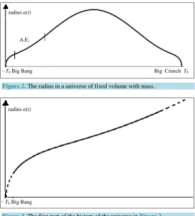
0 = −0.5. In Figure 2 is shown the solution to the Equation (25) with β =1.5 and λ=1.55. In this case, we clearly have a phase of accelerating expansion, i.e. a phase where a t′′( )
>0 (marked with A.E. in the figure). The en-larged picture (Figure 3) shows the early part of the history of this universe, approximately corresponding to the part where we could be right now.On the other hand, the relationship between β and λ turns out to be rather sensitive. I will come back to this in Section 8.
7. An Invariant Motivation for the Gravitational Energy Term
Is there a way of reformulating the approach of the previous section which is invariant and independent of the concept of potential energy?
Big Crunch T0
−T0 Big Bang
radius a(t)
[image:9.595.170.456.399.715.2]A.E.
Figure 2. The radius in a universe of fixed volume with mass.
−T0 Big Bang
radius a(t)
The solution which I suggest is to change the perspective: Instead of considering the curvature of space-time as a kind of mass-energy, perhaps we should instead consider the curvature itself to be the fundamental concept? Thus, what we should do is to try to compute the total amount of curvature (as measured by (6)), caused by the presence of mass in the universe. Then, we should add this to the large scale curvature of the universe itself and minimize the result. In contrast to the potential energy, this total curvature should be a perfectly well-defined and invariant concept.
Of course, if this idea is to make sense, it must be shown that it somehow corresponds to the classical idea of potential energy. To this end, let us consider a very simplified situation.
The metric around a particle or a gravitating body is generally considered to given by the Schwarzschild metric:
1
2 2 2 2 2 2 2
2 2
1 m d 1 m d d sin d
g t r r r
r r σ σ τ
−
= − − + − + +
(26)
There is no reason to doubt that this metric gives an excellent description of the geometry away from the par-ticle. But what happens close to or inside it? This we know very little about. In fact, more or less the only thing we know is that it follows from the field equations that the Ricci curvature must be non-zero there, since there is no global non-singular solution to the field equations Ricci=0 which for large r approaches the Schwarz-schild solution. It also seems very reasonable to assume that for an isolated particle, the amount of curvature present is something which essentially only depends on the particle itself, and in particular is in some sense in-variant along the word-line of the particle. In this case the contribution to the curvature functional Φ in (6) is proportional to the proper time during which Φ is computed, and it is also very natural to assume it to be propor-tional to the mass of the particle.
If we next turn to the case of two particles, what can be said about the curvature then? If the particles are so far away from each other that their interaction can be neglected, then clearly their contributions to Φ will just be the sum of the contributions from the particles separately. This would just add a constant to Φ which would not effect the Euler-Lagrange equation in any way. But if they are still far from each other but close enough to inte-ract, then it is reasonable to treat the total metric as the metric of the vacuum plus two small perturbations caused by the two particles. In particular, as is well-known from general relativity, the presence of one particle with mass m1 contracts the time-scale at the location of the other with mass m2 by a factor
1 1
2
1 m 1 m
r r
− ≈ − (27)
and vice versa. Since the contribution of each particle is proportional to the length of its world-line, it follows that the total (negative) contribution to Φ, caused by the time-contraction, is of the form
1 2
m m r
≈ − (28)
Thus, the conclusion is that the contribution to Φ is of the same form as the classical potential energy which was used in Section 6.
It is important to keep in mind that this argument is based on the idea of a homogeneous gas where the par-ticles interact weakly, and which is so dilute that the total effect can be considered as the sum of all pairwise in-teractions. If the density is higher, the behavior will no longer be additive. Hence, in a universe populated by stars and even super-massive black holes, and in particular near the Big Bang or the Big Crunch, the contribu-tion to Φ could be quite different from what the potential energy approach would give. Nevertheless, for the problem of the accelerating expansion, these considerations may be of less importance. In particular, the plots in Figure 2 and Figure 3 can now be re-interpreted as representing the radius of the closed universe with mass which minimizes the curvature functional Φ in the sense of this section.
Returning to Remark 2, we now also see that with the interpretation in this section, the density ρ now does make sense: is accounts precisely for the amount of curvature as in (6) within the volume element dV which is taken away by the time-contraction caused by all other particles.
Remark 3. It goes without saying that the interpretation of potential energy as curvature in this section is so
abstract level the idea is very simple. But as soon as we want to make computations, the difficulties are enor- mous. On the other hand, making computations with classical potential energy is comparatively easy. Here the problem is instead that on an abstract level we do not really know what we are doing.
My personal opinion is that to compare the predictions that come out of this paper with reality, it is probably quite sufficient to use computations with classical potential energy, just as is done with many other problems in cosmology.
To reach clarity about the connection between this potential energy and the curvature interpretation in this section, the best way is probably computer simulations. In fact, to simulate the metric of a dilute gas and com-pute the corresponding Φ functional is a difficult but probably not impossible problem for a moderate number of particles.
8. The Choice of Parameters
The values of the parameters used to produce the figures of this paper, in particular β, λ and a′′
( )
0 , may appear a little bit arbitrary, and indeed they are. In addition, I have chosen the value of β to be rather large, since this makes the Figure 2 and Figure 3 clearer: a very small value of β would put the region of accelerating expansion close to −T0 in Figure 2 and make it hardly noticeable for the naked eye.I have presently no effective way of determining appropriate values from comparison with the real world. In this section, I will therefor briefly discuss the question whether the chosen values produce typical or non-typical results.
As for the choice of a′′
( )
0 , it seems to be rather innocuous, at least as long as we restrict to the interval]
−1, 0[
. Other choices seem to produce similar graphs for appropriate choices of β and λ. And choices outside this interval are difficult to motivate on physical grounds as remarked earlier. Also, given a value of a′′( )
0 , more or less any value of β >0 again seems to reproduce the characteristic convex phase in Figure 2 for an appropriate value of λ.On the other hand, the relationship between β and λ appears to be rather sensitive: small changes in one of the parameters may result in a solution which looks quite different and in particular may not exhibit the convex be-havior associated with acceleration expansion.
Is this an indication that something is wrong or at least that an accelerating expansion is a rare exception in the kind of models investigated in this paper?
Although I cannot really give a complete answer at the present stage of investigation, there is another expla-nation which I find more plausible. To a large part, the problem is that we are solving the Euler-Lagrange equa-tion in the wrong way. The best way would clearly be to start at the Big Bang and solve forwards in time. This however we cannot do, because we have no good way of stating appropriate initial conditions: such initial con-ditions must by necessity involve more complicated physics than just the metric.
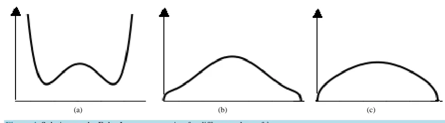
Consider the three graphs in Figure 4, corresponding to the value β =1.5 and λ=1.625, 1.525, 1.425. In the leftmost graph, λ is too big, a t
( )
never reaches the time-axis and the solution diverges. This case does not correspond to any closed universe or, for that part, to any universe which starts with a Big Bang. Thus, such so-lutions do not correspond to any minimizing problem of the kind studied in this paper and can therefore be dis-carded as non-physical.In the graph in the middle we do have a phase of accelerating expansion, but in the rightmost graph, for a somewhat smaller value of λ, there is again no accelerating expansion. Is this behavior physical? As long as we do not have a reasonable theory for what happens at the Big Bang, it is difficult to say. As it seems, the smaller λ gets, the more accentuated the singularity when a t
( )
approaches zero becomes, causing the curvature to di-verge rapidly. Thus it may be that these solutions are non-physical, simply because they generate a super-powerful Big Bang with infinite Φ as in (6). This would clearly contradict the minimizing idea of this paper. For all I know, it may very well be that most of or even all physically acceptable solutions to the global minimizing problem would look essentially like the one in the middle of Figure 4, but the problem is open.9. Discussion
(a) (b) (c)
Figure 4.Solutions to the Euler-Lagrange equation for different values of λ.
should only be considered as an example of possible solutions.
A natural question is whether it is possible to test the model in this paper against observational facts? The answer is yes in principle, but there are problems.
The first problem is that the parameter β is probably, as remarked at the end of Section 5, varying significant-ly during the part of the history of the universe which is accessible for measurements. Even if we roughsignificant-ly iden-tify β as some kind of measure of the potential energy, there still seems to lack adequate estimations of this quantity. This means that the graphs of this paper tend not to be reliable during the early history of the universe.
The second problem is that even if we could estimate the qualitative behavior of β in time, there would still be the problem of comparing the size of it to the global curvature. This can also be expressed by saying that given β, the constant in front of the integral in (6) does not necessarily have to be one. To resolve this is something which inevitably involves the process during which elementary particles generate their gravitational fields, something which we are presently very far from understanding. In theory, it could of course work the other way around too. If we develop this theory and solve the other problems, then it could be that it would eventually give some con-straints on the metric close to individual particles and hence contribute to our understanding of micro-physics. But this is so far just a speculation.
The third problem is that we, except for β, also have the unknown parameters λ and a′′
( )
0 . Data from preci-sion cosmology, in particular from the Planck mispreci-sion, seem to be sufficient to rule out several different possible scenarios and confirm the accelerating expansion. But here the problem is rather the opposite: with three free parameters it seems to be possible to construct so many different graphs a t( )
that some of them will inevitably fit well with the data. But so far this cannot possibly be taken as a confirmation of the theory. However, as mea-surements becomes more and more precise, it can be hoped that eventually we will also be able to separate be-tween all such curves.Also, it should be said that the approach in this paper generates many other questions to which I presently have no answer. One example of such a question is the interpretation of the Lagrange multiplier λ. In usual cos-mology of closed universes, the Lagrange multiplier is typically identified with the cosmological constant. In the context of this paper however, it appears that the cosmological constant will actually be varying with time. So what should we think of the Lagrange multiplier in this situation?
Summing up, it can be said that the minimizing principle in Section 4 gives a possible explanation to the problem with the accelerating expansion of the universe. And in addition, one which does not need any un-known components like dark energy or quintessence. What it demands is instead a reinterpretation of the physics underlying general relativity in terms of very general statistical principles. Still, a lot of work remains in order to understand the theory, and also a lot of work seems to remain before we can really compare the predictions with reality.
References
[1] Bergström, L. and Goobar, A. (2006) Cosmology and Particle Astrophysics. Springer Science & Business Media. [2] Riess, A.G., et al. (Supernova Search Team) (1998) Astronomical Journal, 116, 1009.
http://dx.doi.org/10.1086/300499
[3] Perlmutter, S., et al. (The Supernova Cosmology Project) (1999) Astrophysical Journal, 517, 565. http://dx.doi.org/10.1086/307221
[5] Steinhardt, P.J. and Turok, N. (2002) Science, 296, 1436-1439. http://dx.doi.org/10.1126/science.1070462
[6] Durrer, R. (2011) Philosophical Transactions of the Royal Society A, 369, 5102-5114. http://dx.doi.org/10.1098/rsta.2011.0285
[7] Bean, R. and Tangmatitham, M. (2010) Physical Review D, 81, Article ID: 083534. http://dx.doi.org/10.1103/PhysRevD.81.083534
[8] Parker, S.M.C. (1994) MathTensor: A System for Doing Tensor Analysis by Computer. Addison-Wesley, Reading.
[9] Friedmann, A. (1922) Zeitschrift für Physik, 10, 377-386.
[10] Misner, C.M., Thorne, K.S. and Wheeler, J.A. (1973) Gravitation. W. H. Freeman and Company, San Fransisco.
[11] Wald, R.M. (1984) General Relativity. The University of Chicago Press, Chicago. http://dx.doi.org/10.7208/chicago/9780226870373.001.0001
[12] Einstein, A. (1917) Kosmologische Betrachtungen zur allgemeinen Relativitätstheorie. Sitzungsberichte der Königlich Preussischen Akademie der Wissenschaften.
[13] Dirac, P.A.M. (1975) The General Theory of Relativity. Princeton University Press, Princeton.
[14] Maupertuis, P. (1744)Accord de différentes loix de la nature qui avoient jusqu’ici paru incompatibles. Académie In-ternationale d’Histoire des Sciences, Paris.
[15] Eddington, A.S. (1925) Relativitätstheorie in mathematischer Behandlung. Springer, Berlin.
[16] Pechlaner, E. and Sexl, R. (1966) Communications in Mathematical Physics, 2, 165-175.
[17] Colistete, R. (2002) Constraints on Non-Singular Cosmological Models with Quadratic Lagrangians. arxiv-gr-qc0205024.
[18] Huang, K. (1987) Statistical Mechanics. 2nd Edition, John Wiley & Sons, Inc., New York.
[19] Fischer, H. (2011) A History of the Central Limit Theorem: From Classical to Modern Probability Theory, Sources and Studies in the History of Mathematics and Physical Sciences. Springer, New York.
http://dx.doi.org/10.1007/978-0-387-87857-7