Minimization of Floorplanning Area and Wire Length Interconnection Using Particle Swarm Optimization

(1)

International Journal of Emerging Technology and Advanced Engineering

Website: www.ijetae.com (ISSN 2250-2459,ISO 9001:2008 Certified Journal, Volume 3, Issue 8, August 2013)

321

Minimization of Floorplanning Area and Wire Length

Interconnection Using Particle Swarm Optimization

B Sowmya

1

, Sunil MP

2

1

M.Tech Student, SP and VLSI, 2AssistantProfessor, Department of Electronics and Communication Engineering, Jain University, Karnataka, India

Abstract— Floorplanning is an essential design step for hierarchical building module design methodology. Floorplanning provides early feedback that evaluates architectural decisions, estimates chip area, estimates delay and congestion caused by wiring. As technology advances, design complexity is increasing and the circuit size is getting larger. To cope with the increasing design complexity, hierarchical design and Intellectual Property modules are widely used. This makes floorplanning much more critical to the quality of a Very Large Scale Integration (VLSI) design. For many years, floorplanning is a critical step, as it sets up the ground work for a layout. However, it is computationally quite hard. The process of determining block shapes and positions with area minimization objective and aspect ratio requirement is referred to as floorplanning. Common strategy for blocks floorplanning is to determine in the first phase and then the relative location of the blocks to each other based on connection-cost criteria. In the second step, block sizing is performed with the goal of minimizing the overall chip area and the location of each block is finalized. From the computational point of view, VLSI floorplanning is NP-hard. The solution space will increase exponentially with the growth of circuits scale, thus it is difficult to find the optimal solution by exploring the global solution space. To handle this complexity swarm based optimization method has opted in this proposed work. A generalize solution has developed to take care of area as well as interconnection wire length. To achieve this weighted objective function has defined. The advantages of PSO like simplicity in implementation, not depends upon the characteristics of objective function and better performance have given support to include it as a solution method.

Keywords— Floorplanning, PSO, Matlab Simulation, Area, Wire length.

I. INTRODUCTION

Physical design begins with a floorplan. The floorplan estimates the area of major units in the chip and defines their relative placements. The floorplan is essential to determine whether a proposed design will fit in the chip area budgeted and to estimate wiring lengths and wiring congestion, so an initial floorplan should be prepared as soon as the logic is loosely defined.

Based on the area of the design and the hierarchy, a suitable floorplan is decided upon. Floorplanning takes into account the macros used in the design, memory, other IP cores and their placement needs, the routing possibilities and also the area of the entire design. Floorplanning also decides the IO structure, aspect ratio of the design. A bad floorplan will lead to wastage of die area and routing congestion. To overcome the problem of floorplanning an automated system which taken the input as DFG by the technological help of the PSO has been defined. The problem of the floorplanning has been transferred as a problem of constraint optimization to take care of non overlapping requirement.

The purposed method is not only taking care of required area for the floorplanning but also how to minimize the interconnected wire length is also involved. By considering the following constraints such as:

 Non overlapping constraint: No two modules should overlap.

 Wire length estimation: Wire length between two modules is calculated by calculating the distance between centers of two modules.

 Area Estimation: It‘s the area of rectangle of minimum size, enclosing all the blocks.

 Cost Function & Constraints: A floorplan has an area cost, i.e., which is measured by the area of the smallest rectangle enclosing all the modules and an interconnection cost, i.e., Wire length, which is the total length of the wires fulfilling the interconnections between the modules.

The goal of floorplanning is to optimize a predefined cost function; the floorplan area directly correlates to the chip silicon cost.

(2)

International Journal of Emerging Technology and Advanced Engineering

322

In many design methodologies,areaandspeedare considered to be trade off against each other. The reason is that, there are limited and more routing resources that are used for design. Due to this, designed system will operate slower. Optimizing for minimum area allows the design to use fewer resources, but also allows the sections of the design to be closer together. This leads to shorter interconnect distances, less routing resources to be used, faster end-to-end signal paths, more consistent place and routing times.

The particle swarm optimization (PSO) is an optimization technique inspired by swarm intelligence and theory in general such as bird flocking, fish schooling and even human social behavior. PSO is a population-based evolutionary algorithm in which the algorithm is initialized with a population of random solutions. However, unlike most of other population-based evolutionary algorithms, PSO is motivated by the simulation of social behavior instead of the survival of the fitness. The advantages of PSO over many other optimization algorithms are its simplicity in implementation and its ability to converge to a reasonably good solution quickly. Since the PSO algorithm was proposed, it has aroused great interest among the academic community, massive research results have been presented in only a few years. Hence particle swarm optimization technique will be made use to find the optimal solution for the floorplanning.

II. RELATED WORK

Recently, many researchers resort to stochastic optimization algorithms, such as simulated annealing (Hoet al. 2004), artificial neural networks (Gloria et al. 1994) and tabu search (Handa and Kuga 1995). Genetic algorithm (GA) has been proved to be an effective method for tackling NP-hard optimization problem (Goldberg 1989), and has been successfully applied on VLSI floorplanning problems.

Andrew Kahng, Jens Leinig, Igor L. Markov, Jin Hu, ―VLSI Physical Design: From Graph Partitioning to Timing Closure,‖ Springer, 2011[16]

in this paper, proposed design and optimization of integrated circuits are essential to the creation of new semiconductor chips, and physical optimizations are becoming more prominent as a result of semiconductor scaling.Introduces and compares algorithms that are used during the physical design phase of integrated-circuit design, wherein a geometric chip layout is produced starting from an abstract circuit design. The emphasis is on essential and fundamental techniques, ranging from hyper graph partitioning and circuit placement to timing closure.

Dain Palupi Rini, Siti Mariyam Shamsuddin & Siti Sophiyati Yuhaniz ―Particle Swarm Optimization: Technique, System and Challenges‖. International Journal of Computer Applications (0975-8887), Vol 14-No.1, January 2011[1] according this paper, they have made review of the different methods of PSO algorithm. Basic particle swarm optimization has advantages of PSO. The basic variants as mentioned above have supported controlling the velocity and the stable convergence. At the other hands, modified variant PSO help the PSO to process other conditions that cannot be solved by the basic PSO. The observation and review is made to show the absolute function of PSO, advantages and disadvantages of PSO, the basic variant of PSO, Modification of PSO and applications that have implemented using PSO. The application can show which one the modified or variant PSO that haven‘t been made and which one the modified or variant PSO that will be developed.

S. T. Hsieh, C. W. Lin and T. Y. Sun, ―Particle Swarm Optimization for Macrocell Overlap Removal and Placement,‖ in Proc. of IEEE Swarm Intelligence Symposium (SIS‘05), pp. 177-180, June 2005[7]_{in this} paper proposed a novel algorithm based on the particle swarm optimization (PSO) technique to obtain a feasible macrocell floorplanning without overlaps in VLSI circuit physical placement. The PSO was applied with an overlap detection and removal mechanism in search for optimal placement solution. The proposed PSO exhibited rapidly convergence features and led to more optimal solutions than other approaches.

(3)

International Journal of Emerging Technology and Advanced Engineering

323

Yi-Chun Xu, Ren-Bin Xiao & Martyn Amos ―Particle Swarm Algorithm for Weighted Rectangle Placement‖ [15] according to this paper they present a new algorithm for a layout optimization problem: this concerns the placement of rectangular, weighted objects inside a circular container, the two objectives being to minimize imbalance of mass and to minimize the radius of the container. This problem carries real practical significance in industrial applications (such as the design of satellites), as well as being of significant theoretical interest. They present a particle swarm-based solution and compare it with the best published algorithm for this problem.

III. PARTICLE SWARM OPTIMIZATION ALGORITHM

The particle swarm optimization (PSO), originally introduced by Kennedy and Eberhart [14], is an optimization technique inspired by swarm intelligence and theory in general such as bird flocking, fish schooling and even human social behavior. PSO is a population-based evolutionary algorithm in which the algorithm is initialized with a population of random solutions. However, unlike most of other population-based evolutionary algorithms, PSO is motivated by the simulation of social behavior instead of the survival of the fitness. The advantages of PSO over many other optimization algorithms are its simplicity in implementation and its ability to converge to a reasonably good solution quickly. Since the PSO algorithm was proposed, it has aroused great interest among the academic community, massive research results have been presented in only a few years [9].

The basic PSO algorithm consists of three steps namely, generating particles‘ positions and velocities, velocity update, and finally position update. Here a particle refers to a point in the design space that changes its position from one move (iteration) to another based on velocity updates. First, the positions and velocities , of the initial swarm of particles are randomly generated using upper and lower bounds on the design variables values, xmin and xmax, as expressed in Eq. (1) and Eq. (2) . The positions and velocities are given in a vector format with the superscript and subscript denoting the ith particle at time k. In Eq. (1) and Eq. (2), rand is a uniformly distributed random variable that can take any value between 0 and 1. This initialization process allows the swarm particles to be randomly distributed across the design space [6].

( ) ( ) (

)

( )

The second step is to update the velocities of all particles at time k+1 using the particles objective or fitness values which are functions of the particles current positions in the design space at time k. The fitness function value of a particle determines which particle has the best global value in the current swarm , and also determines the best position of each particle over time pi, i.e. in current and all previous moves. The velocity update formula uses these two pieces of information for each particle in the swarm along with the effect of current motion , to provide a search direction , for the next iteration. The velocity update formula includes some random parameters, represented by the uniformly distributed variables, rand, to ensure good coverage of the design space and avoid entrapment in local optima. The three values that effect the new search direction, namely, current motion, particle own memory, and swarm influence, are incorporated via a summation approach as shown in Eq. (3) with three weight factors, namely, inertia factor, w , self confidence factor, c1 and swarm confidence factor, c2 respectively [8].

( ) ( )

( )

The research presented in this paper found out that setting the three weight factors w, c1, and c2 at 0.5, 1.5, and 1.5 respectively provides the best convergence rate for all test problems considered. Other combinations of values usually lead to much slower convergence or sometimes non-convergence at all.

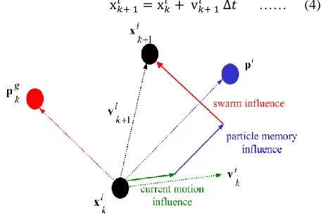
Position update is the last step in each iteration. The Position of each particle is updated using its velocity vector as shown in Eq. (4) and depicted in Fig.1.

[image:3.612.336.564.512.665.2]

…… (4)

(4)

International Journal of Emerging Technology and Advanced Engineering

324

In PSO, the design variables can take any values even outside their side constraints, based on their current position in the design space and the calculated velocity vector. This means that the design variables can go outside their lower or upper limits, xmin or xmax, which usually happens when the velocity vector grows very rapidly; this phenomenon can lead to divergence. To avoid this problem, in this study, whenever the design variables violate their upper or lower design bounds, they are artificially brought back to their nearest side constraint. This approach of handling side constraints is recommended by reference [4] and is believed to avoid velocity ―explosion‖. There has been no recommendation in the literature regarding swarm size in PSO. Most researchers use a swarm size of 10 to 50 but there is no well established guideline.

A.Selection of Parameters for PSO

The main parameters of the PSO model are ω, C1, C2, Vmax and the swarm size S. The settings of these parameters determine how it optimizes the search-space. For instance, one can apply a general setting that gives reasonable results on most problems, but seldom is very optimal. Since the same parameter settings not at all guarantee success in different problems, we must have knowledge of the effects of the different settings, such that we can pick a suitable setting from problem to problem [4].

B. The Inertia Weight ω

The inertia weight ω controls the momentum of the particle: If ω << 1, only little momentum is preserved from the previous time-step; thus quick changes of direction are possible with this setting. The concept of velocity is completely lost if ω = 0, and the particle then moves in each step without knowledge of the past velocity. On the other hand, if ω is high (>1) we observe the same effect as when C1 and C2 are low: Particles can hardly change their direction and turn around, which of course implies a larger area of exploration as well as a reluctance against convergence towards optimum. Setting ω > 1 must be done with care, since velocities are further biased for an exponential growth as shown in Fig.1. This setting is rarely seen in PSO implementation and always together with Vmax. In short, high settings near ‗1‘ facilitate global search and lower settings in the range [0.2, 0.5] facilitate rapid local search.

The decreasing ω-strategy is a near-optimal setting for many problems, since it allows the swarm to explore the search-space in the beginning of the run, and still manages to shift towards a local search when fine-tuning is needed.

This was called PSO-TVIW method (PSO with Time varying inertia weight). According to Eberhart and Shi devised an adaptive fuzzy PSO, where a fuzzy controller was used to control ω over time. This approach is very interesting, since it potentially lets the PSO self-adapt ω to the problem and thus optimizes and eliminates a parameter of the algorithm. This saves time during the experimentation, since fine-tuning of ω is not necessary anymore. At each time-step, the controller takes the ―Normalized Current Best Performance Evaluation‖ and the current setting of ω as inputs, and it outputs a probabilistic change in ω.

C.The Maximum Velocity Vmax

The maximum velocity Vmax determines the maximum change one particle can undergo in its positional coordinates during iteration. Usually we set the full search range of the particle‘s position as the Vmax. For example, in case, a particle has position vector x = (x1, x2, x3) and if −10 ≤ xi ≤ 10 for i = 1, 2 and 3, then we set Vmax = 20. Originally, Vmax was introduced to avoid explosion and divergence. However, with the use of constriction factor χ or ω in the velocity update formula, Vmax to some degree has become unnecessary; at least convergence can be assured without it. Thus, some researchers simply do not use Vmax. In spite of this fact, the maximum velocity limitation can still improve the search for optima in many cases.

D.The Constriction Factor χ

(5)

International Journal of Emerging Technology and Advanced Engineering

[image:5.612.56.277.182.567.2]

325

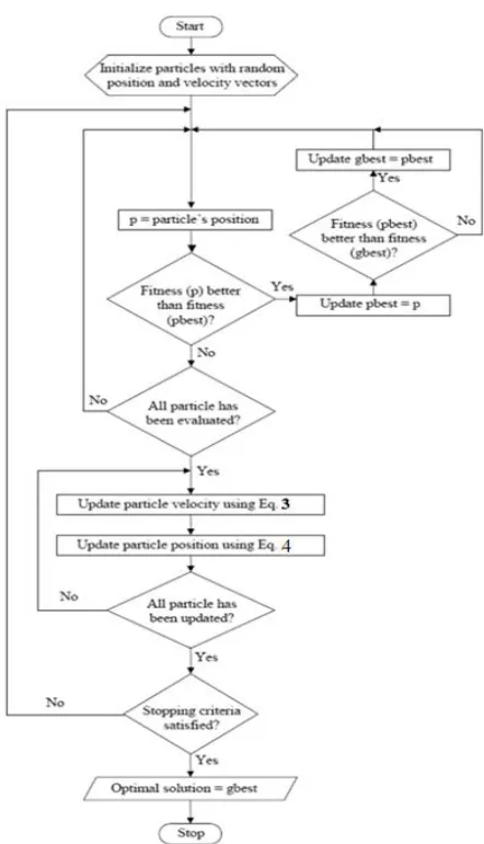
The constriction coefficient method therefore balances the need for local and global search depending on what social conditions are in place. Design flow of PSO is as shown in Fig.2

Fig. 2. Flowchart of particle swarm optimization algorithm

E.The swarm size

It is quite a common practice in the PSO literature to limit the number of particles to the range 20–60. There is a slight improvement of the optimal value with increasing swarm size, a larger swarm increases the number of function evaluations to converge to an error limit.

According Eberhart and Shi [12] illustrated that the population size has hardly any effect on the performance of the PSO method.

IV. FLOORPLANNING USING PARTICLE SWARM

OPTIMIZATION ALGORITHM

[image:5.612.349.538.329.434.2]

During Floorplanning the information is given to a set of macro cells, the information includes their width, length and cell numbers. The goal of proposed method is to plan all macro cells positions on a chip such that nonoverlap constraint can be satisfied and the area and interconnection cost is minimized. In this paper, the notation c(x, y, i) is used to denote the ith cell location, where x and y are ith cell position on x-axis and y-axis respectively. Note that, the cell positions are defined as the cell lower left corner. Fig. 3 illustrates these definitions.

Fig. 3. Cell Definition

Here we are considered 3rd order IIR filter for Floorplanning demonstration using Particle Swarm Optimization algorithm as shown in Fig. 4.

Fig. 4. Third Order IIR Filter

[image:5.612.328.558.484.631.2]

(6)

International Journal of Emerging Technology and Advanced Engineering

326

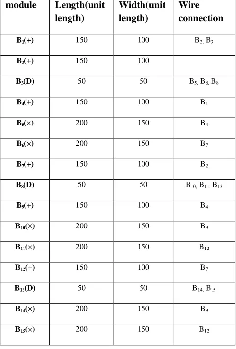
TABLE I

Module description of IIR filter

Module Length Width

Adder 150 100

Multiplier 200 150

[image:6.612.88.247.150.270.2]

Differentiator 50 50

TABLE II

Dimensions of each module with their forward path wire connection

module Length(unit length)

Width(unit length)

Wire connection

B1(+) 150 100 B2, B3

B2(+) 150 100

B3(D) 50 50 B5, B6, B8

B4(+) 150 100 B1

B5(×) 200 150 B4

B6(×) 200 150 B7

B7(+) 150 100 B2

B8(D) 50 50 B10, B11, B13

B9(+) 150 100 B4

B10(×) 200 150 B9

B11(×) 200 150 B12

B12(+) 150 100 B7

B13(D) 50 50 B14, B15

B14(×) 200 150 B9

B15(×) 200 150 B12

A.Non-Overlapping Constraint

Two modules Mi and Mj are nonoverlap, if at least one of the following constraints is satisfied.

Mi to the left of Mj : xi + wi<= xj

Mi below Mj : yi + hi <= yj

Mi to the right of Mj : xi - wj>= xj

Mi above Mj : yi - hj>= yj

Fig. 5. Two modules overlapping

B.Wire length Estimation

Wire length between two modules is calculated by calculating the distances between centers of two modules, which are connected by a forward path, i.e. Euclidean distance between centers of two modules are calculated. Then the overall wire length between the connected modules is added to give the total wire length. Considering Fig. 5 the formula for wire length between centre of modules two Mi and Mj will be:

( ) ∑ ( )

( )

√((

) ( )) (( ) ( )) ( )

Where, cij : connectivity between blocks i and j

dij: Manhattan distances between the centers of rectangles of blocks i and j.

C.Area Estimation

[image:6.612.328.546.170.359.2] [image:6.612.48.289.286.642.2]

(7)

International Journal of Emerging Technology and Advanced Engineering

[image:7.612.64.276.134.276.2]

327

Fig. 6. Area estimation of the given floorplan

Therefore the total area will be

Area (F) = ( ( )– ( )) ( (

)– ( )) ………… (7)

D.Cost Function & Constraints

A floorplan has an area cost, i.e., which is measured by the area of the smallest rectangle enclosing all the modules and an interconnection cost, i.e., Wire length (F), which is the total length of the wires fulfilling the interconnections between the modules. The cost of a floorplan F is defined as follows:

( ) ( ) ( )

( )

w1and w2 are weights assigned to the area minimization objective and the interconnection minimization objective, respectively,

Where 0 ≤ w1, w2≤ 1, and w1 + w2= 1.

Tv is the total overlap violation, which is the total Euclidean distance Between 2 modules which overlap.

E.Fitness Function

The VLSI floorplanning is a minimization problem, and the objective is to minimize the cost of floorplan F, i.e., cost (F).Thus, the fitness of an individual in the population is defined as follows:

( )

( ) ( ) Where, f(x, wh) is the corresponding floorplan of (x, wh), ( ) is the cost of floorplan defined in Eq. (8), x is a matrix which has the (x,y) location of each module and wh is a matrix which has corresponding width and height of each module.

F.Algorithm Description

The steps of the detailed working of PSO algorithm can be described as follows:

Step 1: Load modules data and initial the parameters of the PSO algorithm (such as population size, generations, inertia factor, self confidence, swarm influence, etc.).

Step 2: Generate the initial population, initialize the position and velocity of each particle, and set the pBest of each particle and the gBest population.

Step 3: Calculate the fitness value of each particle with Eq. (9).

Step 4: Check each particle, if its fitness value is better than its pBest, update its pBest with the fitness value.

Step 5: Check each particle, if its fitness value is better than the population‘s gBest, update the gBest with the fitness value.

Step 6: Adjust the position and velocity of each particle according to Eq. (1)-(4).

Step 7: If termination condition is satisfied, the algorithm stops and the inputs which gave gBest fitness is given as output; otherwise, go to Step 3.

[image:7.612.332.555.405.653.2]

(8)

International Journal of Emerging Technology and Advanced Engineering

328

V. EXPERIMENTAL RESULTS

A.Output of 3rd Order IIR Filter

In the floorplanning modules are represented by the set of rectangular blocks which depends upon the module operation. First part of the input represents the dimension of block in terms of length and width. The unit of length defined according to technology applied.

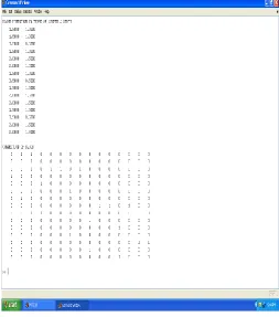
[image:8.612.339.562.146.309.2]

DFG contain interconnection of modules. There is one connection matrix which is defined the connectivity by representing numeric value equal to ‗1‘ in the corresponding row and column position. If there is a ‗0‘ which represents no connectivity as shown in Fig. 8.

Fig. 8. IIR Filter-DFG Connection block

B.Graph of overlap violation

The problem of floorplanning having the constraint of non overlap and these constraints form a set of constraint, which will be included initially. The objective is to minimize the area and wire length.

From the Fig. 9 it is clear that initially because of the random solution there was more violation of constraints and after certain number of iterations PSO discarded all unfeasible solutions.

Fig.9. IIR Filter-Overlap Violation plot with Iteration

C.Graph of area and wire length

From the observation of area minimization plot shown in Fig.10, it is very clear that initially required area for floorplanning is very large but with the iteration it started to decrease and finally become constant that was the indication of no improvement further which suggest the situation for the termination. Same observation has been seen for the total wire length plot shown in Fig.11.

[image:8.612.47.300.296.583.2] [image:8.612.338.552.442.643.2]

(9)

International Journal of Emerging Technology and Advanced Engineering

[image:9.612.63.272.145.326.2]

329

Fig. 11. IIR Filter-Wire length plot with Iteration

From the both graphs Fig. 10 and Fig.11, initially some fluctuation has seen that is because of the process PSO has to optimize the solution whenever there is a complexity associated with the problem. After certain number of iterations there is a smooth optimized process observed.

D.Layout of floor plan

[image:9.612.333.555.179.546.2]

Floorplan result has been observed and it is as shown in Fig.12 which is enclosed by the rectangle with the minimum area which contains all the blocks and is placed in such a manner the wire length could be the minimum.

Fig. 12. IIR Filter-final floorplan layout.

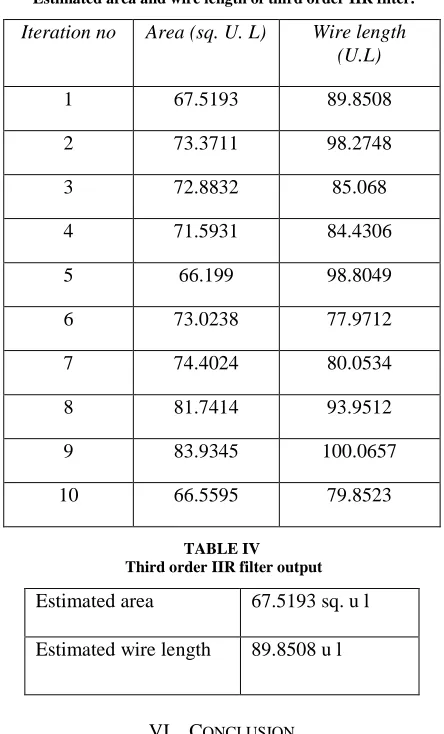
The Results area and wire length are obtained from the tool and that is tabulated in Table III. Here we considered the population size as 200 and 500 number of iteration.

The average area and wire length of third order IIR filter is obtained from the algorithm is tabulated in Table IV.

TABLE III

Estimated area and wire length of third order IIR filter.

Iteration no Area (sq. U. L) Wire length (U.L)

1 67.5193 89.8508

2 73.3711 98.2748

3 72.8832 85.068

4 71.5931 84.4306

5 66.199 98.8049

6 73.0238 77.9712

7 74.4024 80.0534

8 81.7414 93.9512

9 83.9345 100.0657

[image:9.612.332.554.187.548.2]

10 66.5595 79.8523

TABLE IV Third order IIR filter output

Estimated area 67.5193 sq. u l

Estimated wire length 89.8508 u l

VI. CONCLUSION

[image:9.612.59.274.485.658.2]

(10)

International Journal of Emerging Technology and Advanced Engineering

330

The concept of the PSO algorithm has been used because, the number of advantages like, simplicity in the math logic, not much problem dependency and efficient solution.

With the proposed solution we hope that researchers will find a more comfort methodology to obtain the optimal floorplanning and cost effective.

The solution has been proposed in the respect to defining the floorplanning by means of particle swarm optimization; always there is a scope of having some improvement irrespective of what method have applied for solution. In this regard evolutionary programming can be considered as one of the future possibility. A brief description of evolutionary programming has given below. Evolutionary programming (EP) is most widely used approach for optimization problems, which gives the desirable results by using the given constraints to fetch the optimal solution in a reasonable time even when size of the problem increases.

REFERENCES

[1] Dain Palupi Rini, Siti Mariyam Shamsuddin & Siti Sophiyati Yuhaniz ―Particle Swarm Optimization: Technique, System and Challenges‖. International Journal of Computer Applications (0975-8887), Vol 14-No.1,January 2011.

[2] Mohammad Syafrullah, NaomieSalim, ―Improving Term Extraction Using Particle Swarm Optimization Techniques,‖ journal of computing, volume 2, issue 2, february 2010.

[3] Sheng-Ta Hsieh, Tsung- Ying Sun Chan-Cheng-Liu and Cheng-Wei Lin Research article ― An Improved Particle Swarm Optimizer for Placement Constraints‖. Hindawi Publishing Corporation ,Journal of Artificial Evolution and Applications January 2008.

[4] Swagatam Das, Ajith Abraham and Amit Konar. ― Particle Swarm Optimization and Differential Evolution Algorithms: Technical Analysis, Applications and Hybridization Perspectives ‖,Studies in Computational Intelligence 2008.

[5] A review of particle swarm optimization. Part II: hybridization, combinatorial, multicriteria and constrained optimization, and indicative applications‖ By Alec Banks Æ Jonathan Vincent Æ Chukwudi Anyakoha Received: 25 August 2006 / Accepted: 4 June 2007 / Published online: 17 July 2007 Springer Science+Business Media B.V. 2007

[6] Rania Hassan, Babak Cohanim, Olivier de Weck, Gerhard Venter. ―A Comparison of Particle Swarm Optimization and the Genetic Algorithm.‖ AIAA-50; 2005-1897. 46th AIAA/ ASME/ ASCE/ AHS/ ASC Structures, Structural Dynamics and Materials Conference, Austin, Texas, 2005.

[7] S. T. Hsieh, C. W. Lin and T. Y. Sun, ―Particle Swarm Optimization for Macrocell Overlap Removal and Placement,‖ in Proc. of IEEE Swarm Intelligence Symposium (SIS‘05), pp. 177-180, June 2005 [8] Venter, G. and Sobieski, J., ―Particle Swarm Optimization,‖ AIAA

2002-1235, 43rd AIAA/ASME/ASCE/ AHS/ASC Structures, Structural Dynamics, and Materials Conference, Denver, CO., April 2002.

[9] Clarc, M and Kennedy, J (2002). ―The particle swarm – explosion, stability, and convergence in a multidimensional complex space.‖ IEEE Transactions on Evolutionary Computation. pp. 58-73 [10] Kennedy, J., Eberhart, R.C., and Shi, Y.(2001). ―Swarm

Intelligence,‖ San Francisco: Morgan Kaufmann Publishers. [11] Clerc, M. (1999). ―The swarm and the queen: towards a

deterministic and adaptive particle swarm optimization.‖ Proc. 1999 Congress on Evolutionary Computation, Washington, DC, pp 1951-1957. Piscataway, NJ: IEEE Service Center.

[12] Y. Shi and R. Eberhart, ―A modified particle swarm optimizer,‖ in Proceedings of IEEE World Congress on Computational Intelligence, pp. 69–73, Anchorage, Alaska, USA, May 1998. [13] M. Rebaudengo and M. Reorda, ―GALLO: A genetic algorithm for

floorplan area optimization,‖ IEEE Trans. Comput.-Aided Design Integr. Circuits Syst., vol. 15, no. 8, pp. 943–951, Aug. 1996 [14] R. Eberhart and J. Kennedy, ―A new optimizer using particle swarm

theory,‖ in Proceedings of 6th International Symposium on Micro Machine and Human Science, pp. 39–43, Nagoya, Japan, October 1995.

[15] Yi-Chun Xu, Ren-Bin Xiao & Martyn Amos ―Particle Swarm Algorithm for Weighted Rectangle Placement