The implications of judgemental interventions into an inventory System

(1)

THE IMPLICATIONS OF JUDGEMENTAL

INTERVENTIONS INTO AN INVENTORY

SYSTEM

Inna KHOLIDASARI

(2)

THE IMPLICATIONS OF JUDGEMENTAL

INTERVENTIONS INTO AN INVENTORY

SYSTEM

Inna KHOLIDASARI

Salford Business School

College of Business & Law

University of Salford, Salford, UK

Submitted in Partial Fulfilment of the Requirements

Of the Degree of Doctor of Philosophy

(3)

i

List of Figures

Figure 1.1 The incorporation of human judgement into an inventory system ... 3

Figure 1.2 The organisation of the thesis ... 9

Figure 2.1 An overview of a typical inventory system ... 11

Figure 2.2 Williams’ categorisation scheme ... 15

Figure 2.3 Eaves’ categorisation scheme ... 16

Figure 2.4 Syntetos and Boylan categorisation scheme ... 18

Figure 3.1 Classification of methodology in operation management research. ... 66

Figure 3.2 Theoretical framework of the research ... 73

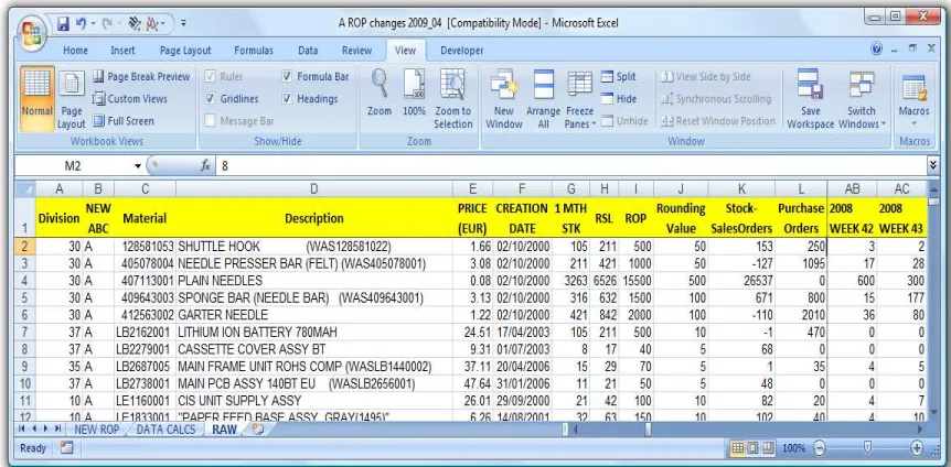
Figure 4.1 RAW sheet of original data ... 79

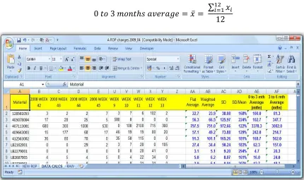
Figure 4.2 Data calculation sheet for original data ... 82

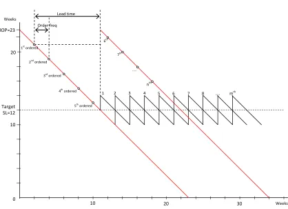
Figure 4.3 Stock control system for A items ... 83

Figure 4.4 Stock control system for B items ... 83

Figure 4.5 An example of the adjustment process ... 86

Figure 4.6 The process of adjustments to the OUT level. ... 86

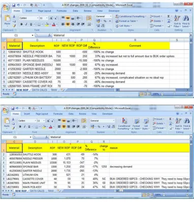
Figure 4.7 NEW ROP sheet of original data ... 87

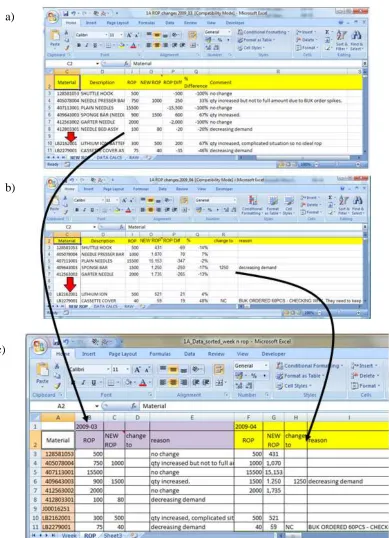
Figure 4.8 Compiling information into a time-series format ... 88

Figure 4.9 Complete database over time ... 89

Figure 4.10 Weekly demand data for whole time horizons ... 90

Figure 4.11 Original data of detailed OUT level ... 91

Figure 4.12 Detailed ROP for whole time horizons ... 92

Figure 4.13 Complete database for A items ... 93

Figure 4.14 Philosophical positioning of the research ... 104

Figure 4.15An integrated (semi-deductive) research approach ... 105

(9)

vii

Figure 4.17 Research choices ... 108

Figure 4.18 The research onion of this work ... 111

Figure 5.1 The distribution of average inter-demand interval for A items. ... 114

Figure 5.2 Distribution of material price for A items ... 117

Figure 5.3 Distribution of material price for B items ... 117

Figure 5.4 Distribution of the signed size of adjustments for A items ... 121

Figure 5.5 Distribution of the absolute size of adjustments for A items ... 122

Figure 5.6 Distribution of the relative signed size of adjustments for A items ... 122

Figure 5.7 Distribution of the relative absolute size of adjustments for A items ... 123

Figure 5.8 Distribution of the signed size of adjustments for B items ... 124

Figure 5.9 Distribution of the absolute size of adjustments for B items ... 124

Figure 5.10 Distribution of the relative signed size of adjustments for B items ... 125

Figure 5.11 Distribution of the relative absolute size of adjustments for B items ... 125

Figure 5.12 Slope of demand pattern ... 128

Figure 5.13 Comparison between trends and reason for judgement made by manager 129 Figure 5.14 Example of inconsistency (the reason for making an adjustment is ‘decreasing demand’ while the demand is increasing over time) ... 130

Figure 5.15 Example of inconsistency (the reason for making an adjustment is ‘increasing demand’ while the demand is decreasing over time) ... 130

Figure 5.16 Distribution of adjustments per justification category (A items) ... 132

Figure 5.17 Distribution of adjustments per justification category (A items) ... 133

Figure 5.18 Verification and validation of the simulation model ... 138

(10)

viii

List of Tables

Table 3.1 Comparison of the Traditional and the New Paradigm ... 66

Table 3.2 Model assumptions and possible behavioural gaps in inventory and supply chain management. ... 68

Table 3.3. Function of MM sub-menus. ... 71

Table 4.1 Classification of main types of research ... 100

Table 4.2 Contrasting positivist and interpretivist ... 103

Table 4.3 Relevant situations for different research methods ... 107

Table 4.4 Dimension of contrast among the three research choices ... 109

Table 5.1 Demand data series characteristics for A items ... 113

Table 5.2 Demand data series characteristics for B items ... 113

Table 5.3 Spare parts prices for A items and B items. ... 115

Table 5.4 Theoretical distributions being tested ... 120

Table 5.5 Adjustment distributions for A items and B items. ... 126

Table 5.6 Number of adjustments per justification category(A items) ... 131

Table 5.7 Number of adjustments per justification category(B items) ... 132

Table 5.8 The simulation results for A items ... 140

Table 5.9 The simulation results for B items ... 140

Table 5.10 The effect of sign adjustments on inventory performance for A items ... 143

Table 5.11 The results of sign adjustments on inventory performance for B items ... 143

Table 5.12 The results of absolute of adjustment on the inventory performance analysis for A items ... 148

(11)

ix Table 5.14 The results of absolute signed of adjustments on the inventory performance

analysis for A items ... 151 Table 5.15 The effects of absolute signed of adjustments for B items ... 151 Table 5.16 The results of justification of adjustments on the inventory performance

analysis for A items ... 155 Table 5.17 The results of justification of adjustments on the inventory performance

analysis for B items ... 155 Table 5.18 The results of the bias of adjustments on the inventory performance analysis for A items ... 160 Table 5.19 The results of the biased on adjustments on the inventory performance

analysis for B items ... 160 Table 5.20 The results of learning-effects analysis based on number of adjustments for

A items ... 163 Table 5.21 The results of learning-effects analysis based on number of adjustments for

B items ... 163 Table 5.22 The simulation results for A and B items ... 167 Table 5.23 Data of SMA-based OUT replenishment levels and Final OUT

(12)

x

Abstract

Physical inventories constitute a considerable proportion of companies’ investments in today’s competitive environment. The trade-off between customer service levels and inventory investments is addressed in practice by formal quantitative inventory management (stock control) solutions. Given the tremendous number of Stock Keeping Units (SKUs) that contemporary organisations deal with, such solutions need to be fully automated. However, managers very often judgementally adjust the output of statistical software (such as the demand forecasts and/or the replenishment decisions) to reflect qualitative information that they possess. In this research we are concerned with the value being added (or not) when statistical/quantitative output is judgementally adjusted by managers. Our work aims to investigate the effects of incorporating human judgement into such inventory related decisions and it is the first study to do so empirically. First, a set of relevant research questions is developed based on a critical review of the literature. Then, an extended database of approximately 1,800 SKUs from an electronics company is analysed for the purpose of addressing the research questions. In addition to empirical exploratory analysis, a simulation experiment is performed in order to evaluate in a dynamic fashion what are the effects of adjustments on the performance of a stock control system.

(13)

xi

Acknowledgements

I would like to thank the following people and organisations for supporting me in numerous ways throughout my PhD.

First and foremost, I would like to express my wholehearted gratitude to Prof. Aris A. Syntetos, my supervisor, for his patience and his constant support and guidance throughout the period of my Ph.D. study.

I would like to thank the Ministry of National Education and Culture, Government of Indonesia, for providing the scholarship for my Ph.D and the Salford Business School, University of Salford for all the support and facilities.

Special thanks to my friends in Maxwell 528, Dima, Wenjia, Asif, Ila, Rossi, Katie, Afaf and Sira for all their wonderful friendship during the last four years. Many thanks to my best friend Dave, the one who knows what I need more than myself.

Also, many thanks and love to my family; Ibu, Bapak, Mama, Papa, Dhida, Yanna, Affan for all their love, encouragement and for always praying for me.

(14)

xii

Dedication

(15)

xiii

Declaration

This thesis is submitted under the University of Salford requirements for the award of a PhD degree by research. Some research findings were published in refereed conference proceedings prior to the submission of the thesis during the period of PhD studies. The researcher declares that no portion of the work referred to in the thesis has been submitted in support of an application for another degree or qualification to the University of Salford or any other institution.

(16)

1

Chapter 1. INTRODUCTION

1.1. Outline

This research is concerned with the effects of incorporating human judgement into inventory-related decisions. In particular, we1 focus on the case of service/spare parts inventories. This introductory chapter describes the motivation behind this research by placing the study in a business context. Section 1.2 discusses the research background, followed by the need for the research in Section 1.3. The aim and objectives of the research are given in Section 1.4. Finally, Section 1.5 focuses on the structure of this thesis.

1.2. Research background

Physical inventories constitute a considerable proportion of companies’ investments in today’s competitive environment. According to the 22nd Annual State of Logistics Report, the world is currently sitting on approximately $8 trillion worth of goods held for sale (Wilson, 2011). About 10% of that value relates to spare parts; according to US Bancorp, spare parts relate to a $700 billion annual expenditure, constituting about 8% of the US gross domestic product (Jasper, 2006). Mobley (2002) argues that maintenance costs typically account for 15-60% of the total value of an end product, validating the figures presented above with regards to spare parts expenditure. The following statistics are also relevant: two relatively recent reports by the Aberdeen Group (2005) and Deloitte (2006)

1_{The use of the word “we” throughout the thesis is purely conventional. The work presented in this PhD}

(17)

2 identify the increasing importance of the spare parts business. As stated in the latter report, the combined revenues of many of the world's largest manufacturing companies are more than US$1.5 trillion. Furthermore, on average, service revenues account for more than 25% of the total business. To the best of our knowledge, such figures have not been published for the United Kingdom alone, but based on the above it is clear that small improvements regarding the management of maintenance and of spare parts may be translated into substantial cost savings, with a considerable contribution to the country’s economy.

(18)

3 boundaries of SKU classification in an arbitrary way (e.g. William, 1984; Eaves, 2002), despite the existence of more logically coherent approaches such as those proposed by Johnston and Boylan (1996) and Syntetos and Boylan (2005). Even more frequently, they judgementally adjust a statistical forecast or a replenishment decision. If, for example, the forecast produced by the system for a particular SKU is 10 units, then a manager may introduce some qualitative information and amend the forecast to, say, 15 units, thus overriding the system. Similarly, a replenishment decision of 15 units may be reduced to reflect additional information available to the manager, about, for example, some increased competition (due to a competitor reducing their prices) likely to occur in the near future. The process discussed above is depicted in the following figure (Figure 1.1).

Figure 1.1 The incorporation of human judgement into an inventory system

Although there is a growing body of empirical knowledge in the area of judgementally adjusting statistical forecasts, there has been little discussion about judgemental adjustments neither to SKU classification; nor at the moment there a single empirical study that explores the effects of such judgemental adjustments into replenishment decisions. This is most important in terms of developing our understanding of the process of training provision and design of decision support systems. All these issues are discussed later on in this thesis in more detail.

Inventory system

Forecasting Classification of

SKUs

Stock control

Judgement

Stock holding cost CSL

(19)

4

1.3. Need for the research

Because of the tremendous number of SKUs that both manufacturing and service organisations deal with, it is clear that the inventory task needs to be automated. Automation here implies fully quantitative models that can run on their own without human intervention, thus relying upon statistical, generalisable principles. Such models rely upon past information that is available to the system and thus may not of course capture contextual knowledge that managers may possess. For example, experts/managers may know that institutions are in the process of change, or that a product promotion is about to take place, that certain actions are being undertaken by competitors that will affect demand for the product, or that a manufacturing problem exists. The impact of these events is specific, and cannot be included in the model being used. Similarly, a variable that is difficult to measure may be missing from the model. Judgement may be used when insufficient data is available to support statistical methods, or situations arise where exceptional events are known to be occurring in the future. In practice, managers adjust the output of automated systems by altering some quantities, and this is not necessarily a bad thing. As Soergel (1983) and Jenks (1983) pointed out, it is judgement alone that can anticipate one-time events which, if not accounted for, could have severe negative consequences for the organisation.

(20)

5 21% did so frequently. Furthermore, 45% of the respondents said that they always adjusted their statistical forecasts and 37% did so sometimes. In a study of Canadian firms, Klassen and Flores (2001) reported that 80% of the respondents that used computer-based forecasts used judgement to adjust them.

A plethora of studies look at this phenomenon in regards to forecasting. However, in terms of inventory systems, practitioners often adjust the stock replenishment order, not the forecast. Kolassa et al. (2008) report that judgemental adjustments of stock control quantities occurs more often than forecast-related adjustments.

A distinction needs to be made at this point between: i) solely employing judgement as a means of predicting the future, and ii) the use of quantitative methodologies adjusted by managers in order to reflect qualitative information. In this research we refer to the latter, and although there are numerous studies that look at this phenomenon when it comes to forecasting, there are no studies at all that examine: i) the effects of judgementally adjusting classification rules, ii) the effects of judgementally adjusting replenishment decisions, and iii) the cumulative effect of adjusting more than one aspect of the system under concern. In this research we are concerned with the effects of judgement on replenishment decisions.

(21)

6 reported that this field of study should be very much associated with inventory management and production management; however, this is the first study that attempts to do so and currently (and as discussed above), to the best of our knowledge, there is not a single paper in the academic literature that addresses this issue.

We do so by means of analysing an extended empirical database coming from the electronics industry. Managers in the company under consideration adjust inventory quantities, often providing a qualitative justification for their action. Linking the effects of adjustments to the justification provided for such adjustments has never been discussed in the academic literature before; this linkage (on its own) is perceived as a major contribution of the thesis.

The fact that this work is based on a single case can be justified partly by the lack of any previous research in this area, but mostly on the sensitivity of the information required to perform such a study. Adjustments reflect a manager’s personal opinion and such data cannot be easily retrieved. In addition, and as will be explained later in this report, the very construction of the database was a very difficult exercise since the company provided only fragmented information which needed to be constructively put together.

(22)

7 database available for the purposes of this research relates to service parts, there is a safe extension of our discussion and findings to all intermittent demand products.

1.4. Aim and objectives

This study aims to explore the effects of incorporating human judgement into inventory decision-making. From a theoretical perspective there is tremendous scope for contributing and further advancing the current state of knowledge, since there have been no studies addressing this issue to date. From a practitioner’s perspective, the findings of this research result into tangible suggestions and recommendations to inventory managers of service parts and beyond, in addition to the obvious implications for decision support systems design and improvement.

The aim of the research is reflected in the following objectives:

1. To critically review the literature on how judgement relates to the main functions of an inventory system.

2. To assess the implications of judgemental adjustments on real data, focusing on replenishment orders.

3. To link the performance of adjustments with the managers’ justification for introducing such adjustments in the first place.

4. To understand for the first time how managers adjust inventory-related decisions. 5. To evaluate the circumstances under which human judgement leads to performance

improvement.

(23)

8

1.5. The structure of the thesis

The remainder of this thesis is organised as follow:

Chapter 2 provides a literature review of issues related to demand categorisation, forecasting and stock control. Each element of the inventory management system is presented under a separate section of the chapter. The literature review focuses on the intermittent demand context since the empirical data used in this research relates to service/spare parts. Such SKUs are known to be almost invariably characterized by intermittent demand structures.

In Chapter 3 the issue of judgemental adjustments into an inventory system is discussed. The relevant part of the forecasting literature is widely reviewed along with the very few contributions that have emphasized demand categorisation as well as stock control. This chapter also discusses learning and forgetting effects in the manufacturing domain (because of its relevance to the focus of this research), and presents a state of the art into the new paradigm of inventory management. Information about enterprise resource planning (ERP) systems is also provided as this links to the case organisation. The company under concern perform inventory management under an ERP solution and in that respect a clear understanding of how such solutions operate (in particular with regards to inventory management) is viewed as imperative to provide. Finally, a theoretical framework for this research is also presented.

Chapter 4 outlines the case organisation, the construction of the empirical database used for experimentation purposes and the research questions developed to guide the experimental part of the empirical investigation. The research methodology is also discussed in detail in this chapter.

(24)

9 discussed. A simulation experiment is developed for the purpose of addressing the research questions.

Finally, Chapter 6 focuses on the conclusions of this research, implications of our work for real world practices, the limitations associated with our research and important avenues for further work in this area.

[image:24.595.96.517.273.626.2]

The organisation of this thesis is pictorially represented in Figure 1.2.

Figure 1.2 The organisation of the thesis

Chapter 3:

Judgemental adjustments in an inventory system Chapter 2:

An overview of inventory systems

Chapter 4:

Empirical data and research methodology

Chapter 5: Empirical data analysis

Chapter 1:

Background and the need for the research

Chapter 6:

(25)

10

Chapter 2. AN OVERVIEW OF

INVENTORY SYSTEMS

2.1. Introduction

This chapter sets the context of our investigation by presenting an overview of the typical operation of an inventory system. Issues related to judgemental adjustments in such a system are discussed in detail in Chapter 3.

(26)

[image:26.595.144.494.66.364.2]

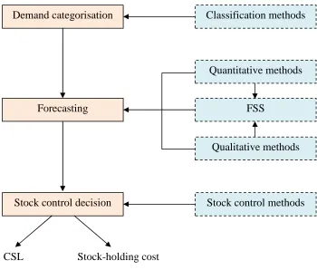
11 Figure 2.1 An overview of a typical inventory system

Demand classification methods have been extensively discussed over the years (by, for example, Johnston and Boylan, 1996; Eaves, 2002; Syntetos and Boylan, 2005 and Teunter et al. 2010; we return to this issue in sub-sections 2.2.1 and 2.2.2 to discuss in detail methods of demand classification). The purpose of demand categorisation2 is to decide on the appropriate forecasting and inventory control methods to be used for each selected category to extrapolate requirements into the future and decide on replenishments actions respectively. With regards to the forecasting task in particular, systems to support or facilitate such a task (forecasting support systems, or FSS) have also been developed to improve the performance of forecasting (selection of quantitative methods or indication of the need for qualitative input). The output of the forecasting process constitutes the input into stock control systems. For the performance of the entire system is then typically reflected into two main things: inventory costs and service levels achieved.

2

The words ‘categorisation’ and ‘classification’ are used interchangeably in this thesis. Demand categorisation

Forecasting

Stock control decision

Qualitative methods

Stock control methods FSS

Quantitative methods Classification methods

(27)

12 In an inventory system, every stage (demand classification, forecasting, and stock control decision-making) maybe completely automated, or parts of the process may be decided or adjusted by managers. For example, a manager may impose particular categorisation criteria and cut-off values, while the forecasting and stock control tasks are fully optimised by the software in use. Alternatively, the software may be used to determine demand categorisation and stock control decisions while forecasting operates in a semi-automated fashion with judgemental adjustments; and all the combinations thereof. Furthermore, both the tasks of forecasting and inventory control introduce various possibilities for human intervention. Managers may intervene in the process of selecting the methods, or the parameters of the methods to be used or both, in addition of course to directly adjusting directly the forecasts or replenishment decisions themselves. In this research we are concerned with the intervention in the final output of the system.

2.2. Demand categorisation

(28)

13 2.2.1.ABC classification scheme

Demand can be classified according to a number of factors, such as the underlying demand characteristics, criticality, and cost. One common type is the ABC (Pareto) classification scheme. Silver et al. (1998) explained that a Pareto report lists the SKUs in descending or ascending order based on demand frequency, demand volumes or demand profit, and then divides the ranked SKUs into relevant categories. Category A is assumed to consist of the most important SKUs and therefore requires the highest service level, category B contains SKUs of moderate importance, and relatively unimportant SKUs are placed in category C (Lengu, 2012). However, in the spare/service parts context, the C items may become an important or critical category if managers consider the carrying cost of such items within the inventory. As the majority of spare/service parts are demanded in relatively low quantities in every period (less than once per month: Teunter et al., 2010) and because obsolescence is highly likely, such items may indeed end up being more important than A items.

ABC classifications based on demand frequency/volume are often used in conjunction with other criteria; the value (SKU cost × quantity required) criterion is the most commonly applied one. Originally, the ABC classification was designed for three classes; the method can, however, be extended to include more. For example, Syntetos et al. (2009a) addressed the issue of demand classification for the purpose of suggesting forecasting and stock control policies for increasing service levels and reducing stock-holding costs in an after-sales business context. This study investigated data from a manufacturing company which initially classified its products into six categories, based on demand frequency.

(29)

14 process technology, and substitutability (see e.g. Flores and Whybark, 1987; Partovi and Burton, 1993; Buzacott, 1999; Ramanathan, 2006; Ng, 2007; Zhou and Fan, 2007; Chen et al., 2008). Moreover, various multi-criteria methodologies have been considered, including weighted linear programming, the analytic hierarchy process (AHP), and operation-related groups (ORG). An alternative to multi-criteria methodologies is to use multiple way classification, e.g. a two-way classification by purchase cost and demand value (Teunter et al., 2010).

2.2.2.Demand characteristics

SKUs can be classified into relevant groups based on the characteristics of demand (for example, number of orders for a particular period, demand size, and lead time between demands). We now examine a number of studies which discuss various categorisation procedures based on demand characteristics.

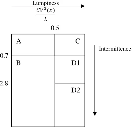
Williams (1984) proposed classification methods (for constant and variable lead time) based on the variance of demand during lead time (DDLT). The variance of DDLT is composed from three factors: the number of orders, the demand size of these orders and the length of the lead times. By considering the mean lead time , the mean demand arrival

(30)

[image:30.595.198.416.74.287.2]

15 Figure 2.2 Williams’ categorisation scheme

(source: Williams, 1984, pp. 942)

The intermittence of demand is indicated by . The higher the ratio, the more intermittent

demand is. indicates the lumpiness of demand. The higher the ratio, the lumpier demand is. Lumpiness depends on the intermittence and variability of the demand sizes. The

classified into three categories using the parameters and : category A, and C - smooth; category B - slow moving; category D1- sporadic; category D2- highly sporadic.

Two demand categorisation methods for non-constant lead times were developed from this study. The first is constructed based on the size of the three summand factors discussed above, and classifies demand into smooth, slow-moving, sporadic, and sporadic with highly variable lead time. The second method assumes that in any lead time, demand has a probability of being zero (p) and if it is non-zero, it equals a random variable (y). The product is classified using p and (squared coefficient of variation of non-zero demand) as slow-moving demand if p>0.25 and ≤0.4 and sporadic demand if p>0.7 and c >0.4. This study did not intend to develop a generalised solution as the break-point values used for the categorisation parameters were decided based on the characteristics of the particular

A C

D1

D2 B

Intermittence 0.7

2.8

0.5

( )

(31)

16 sample used in the study. It is therefore questionable whether this classification would be effective when used to classify SKUs in other datasets. In addition, these break-points are defined without considering the relative performance of different forecasting methods and inventory policies.

Eaves (2002) developed a demand pattern classification scheme based on three lead time demand components discussed above: i) transaction variability, ii) demand size variability, and iii) lead-time variability. This study used demand data from the Royal Air Force (RAF) and found that it was not sufficient to distinguish a smooth demand pattern simply on the basis of transaction variability. Figure 2.3 shows the Eaves categorisation scheme (that evolved from that developed by Williams, 1984) which divides demand patterns into smooth (category A), slow-moving (category B), irregular (category C), erratic (category D1), and highly erratic (category D2). The cutoff values were decided based on the characteristics of the particular demand dataset and sufficient sub-sample size considerations. The cut-off points were as follows: transaction variability: 0.74; demand size variability: 0.10; lead time variability: 0.5.

Figure 2.3 Eaves’ categorisation scheme (source : Eaves, pp. 127)

A C

D1

D2 B

Lead-time variability 0.74

0.53 0.10

Demand size variability

(32)

17 The objective of the demand categorisation methods of the above two studies was to define the appropriate forecasting and inventory control methods for the resulting categories. The boundaries of the demand categories were determined arbitrarily by the managers at which point estimation procedures and stock control methods were selected in order to forecast future requirements and manage stock efficiently.

Syntetos and Boylan (2005) established a more logical approach than that presented above, based on the work conducted by Johnston and Boylan (1996). The demand categorisation procedures suggested rely on the premise that is preferable to first compare alternative forecasting (and stock control) methods for the purpose of establishing regions of superior performance and then classify the SKUs based on the results. That is, if the purpose of demand classification is indeed to select the most appropriate forecasting and stock control methods, then we should start from these methods and by means of comparing them identify regions of superior performance. Classification then naturally follows in a meaningful manner. The work of Johnston and Boylan (1996) considered simulated Mean Squared Errors for the purpose of comparing alternative forecasting methods (Croston’s method (Croston, 1972) and Single Exponential Smoothing, SES) resulting in the identification of the average inter-demand interval as an important classification parameter (to distinguish between intermittent and non-intermittent demand). Syntetos and Boylan (2005) took this work further by means of analysing theoretical MSE expressions and identifying an additional classification parameter that relates to the variability of the demand sizes, when demand occurs. The rule proposed was empirically validated on 3,000 intermittent demand series from the automotive industry.

(33)

[image:33.595.129.445.146.362.2]

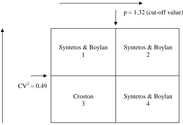
18 were: Croston, SES and the Syntetos-Boylan Approximation (Syntetos and Boylan, 2005). The rule results in a four-quadrant solution presented in Figure 2.4.

Figure 2.4 Syntetos and Boylan categorisation scheme (source: Syntetos et al., 2005, pp. 500 )

There is a direct suggestion now of the forecasting method to be used in each category. In addition, the cut-off points are the outcome of a generalised analytical comparison (albeit under specific modeling assumptions).

Kostenko and Hyndman (2006) revisited the categorisation procedure proposed by Syntetos and Boylan (2005) in terms of some approximate simplifying assumptions that permitted the easy four-quadrant approach presented above, and suggested a linear function for separating between Croston and the Syntetos-Boylan Approximation (which is discussed in detail sub-section 2.3). Heinecke et al. (2013) conducted a simulation experiment to empirically investigate the performance of the above discussed procedures using more than 10,000 SKUs from three different industries (electronics, military, and automotive). The results indicated that the categorisation scheme proposed by Kostenko

Syntetos & Boylan 1

Syntetos & Boylan 2

Croston 3

Syntetos & Boylan 4

p = 1.32 (cut-off value)

(34)

19 and Hyndman (2006) performed well but it is questionable whether the small gains in accuracy improvement worth the additional complexity of the scheme.

Syntetos et al. (2009a) conducted a study on demand categorisation for a European spare parts logistics network, in order to facilitate decision making with respect to forecasting and stock control, and to enable managers to focus their attention on the most important SKUs. This research considered the cumulative demand frequency versus cumulative demand value (demand value = SKU cost × quantity required) as a demand classification parameter. This scheme resulted in six categories of items with each category being associated with a specific treatment in terms of forecasting and stock control.

Syntetos et al. (2010a) suggested that it is important for organisations to classify their SKUs in order to assign higher service-level targets to some critical-item categories and identify obsolete SKUs that are very slow moving. In that study, the researchers conducted a demand categorisation of 2,156 SKUs using the ABC (Pareto) classification based on their contribution to profit (sales volumes × net profit). The results revealed the scope for improving the system through increased managerial attention to the best selling items and also to obsolete SKUs.

2.3. Forecasting

(35)

20 no demand at all. The latter is also known as an intermittent demand pattern (Silver et al., 1998; Syntetos and Boylan 2001; 2005; 2006; Willemain et al., 2004).

Many forecasting procedures for fast-moving items have developed and are regarded as well established methodologies. These are commonly based on the assumption that demand follows the normal distribution. However, this assumption is inadequate when the forecasting method is applied to an intermittent demand pattern, since such demand occurs sporadically, sometimes with a high variability of demand size (i.e. a lumpy demand pattern). Numerous studies have considered the statistical distribution of intermittent demand items. Syntetos et al. (2012) conducted goodness-of-fit tests of various statistical distributions (Poisson, Negative Binomial Distribution [NBD], Stuttering Poisson, Normal, and Gamma) by employing the Kolmogorov-Smirnov test, and investigated the implications of particular distributions on the stock control performance. Three empirical spare parts datasets were used for the empirical analysis and it was found that the Negative Binomial Distribution (NBD) performs best in an inventory context.

(36)

21 (Porras and Dekker, 2008; Nikolopoulos et al., 2011). In the following section, we will discuss intermittent demand procedures as these methods are relevant to the empirical data used in this research, whereas a discussion of forecasting methods for fast-moving demand can be found in Appendix A.

2.3.1.Quantitative methods

Quantitative methods are based on algorithms of varying complexity to analyse historical data typically available in a time series format for the specific variable (s) of interest. Most commonly, this means that a time series of demand information is available and analysed for the purpose of extrapolating requirements into the future. Quantitative forecasting methods are used when sufficient information is available and when it may be reasonably assumed that whatever happened in the past will also persist into the future. The word ‘sufficient’ needs of course to be qualified. This depends on which method is to be employed. For example, if we are to consider a seasonal forecasting method then a few years of complete histories of demand need to be available in order to estimate the annual seasonal pattern.

The estimation procedures typically used in the area of intermittent demand can be divided into two categories (Lengu, 2012): i) the methods that estimate the mean demand level directly (e.g. single exponential smoothing (SES) and simple moving average, or SMA), and ii) those that build demand-level estimates from constituent elements (e.g. Croston’s method, Syntetos and Boylan Approximation or SBA).

2.3.1.1.Simple Moving Average (SMA)

(37)

22 observation is dropped and the most recent one is included (Makridakis et al., 1998). Sani and Kingsman (1997) conducted a simulation study that compared various forecasting methods (including Croston method and SMA). Their analysis used multiple criteria (cost and service level), and found that SMA provided the best overall performance.

2.3.1.2.Exponentially Weighted Moving Average (EWMA)

Exponentially Weighted Moving Average (EWMA) or Single Exponential Smoothing (SES) is perhaps the most commonly used method in an intermittent demand context due to a combination of its simplicity and robustness (Willemain et al., 2004). This method implies the assignment of exponentially decreasing weights as the observations get older, and updates estimates in every inventory review period whether or not demand occurs during this period (Makridakis et al., 1998). (Other forms of exponential smoothing have been developed for demand patterns that may contain trend and/or seasonal components. Intermittent demand may indeed be associated with such components which are impossible though to identify due to the presence of zeroes. As such we rely upon level type methods.) If is the demand during period t, then the SES estimate of demand during period t + 1 (product at the end of period t) is given by

= + = + (1 − )

where α is the smoothing constant value used (0<α<1) and et the forecast error in period t.

2.3.1.3.Croston’s method

(38)

23 applied to each of the constituent series by updating only at the end of demand occurring periods. The following notation is used to define Croston’s method mathematically:

= =demand for an item at time t = size of demand

= binary indicator of demand at time t "_{= Croston’s estimate of mean demand size}

"_{= Croston’s estimate of mean interval between demands}

q = time interval since last demand

= smoothing parameter If

= 0

" ₌ "

" ₌"

" = " + 1

else

" ₌ " _{+ # −} " _$

" ₌" _{+ #" −}" _$

" = 1

Combining the estimates of size and interval provides the estimate of mean demand per period:

(39)

24 The method updates the estimates after demands occur; if a review period t has no demand, the method just increments the count of time periods since the last demand with no updating.

Croston assumed demand to occur as a Bernoulli process, rendering the intervals between demands independent and identically distributed, with the demand sizes also being assumed to be independent and distributed based on the normal distribution.

Croston’s concept has been claimed to be great value for manufacturer that deal with intermittent demand and available in ERP type solution (Syntetos and Boylan, 2001; Teunter et al., 2011). However, this method has disadvantages as it is positively biased since the demand size and the inter-demand interval ratio fail to produce accurate estimates of demand per time period (Syntetos and Boylan, 2001). The biased is true for all point in time and issue points only. Moreover, Croston procedure is not updating after periods with zero demand renders the method unsuitable for dealing with obsolescence issue (Teunter et al., 2011).

Leven and Segerstedt (2004) presented a modification of the Croston method which can be applied to both fast-moving and slow-moving items and, according to them, can be useful as a practical forecasting method. The modified Croston (MC) for mean demand is as follows:

()* = ()* + +_- ,*

*− -* − ()* .

where n = is an index counting the periods in which demand occurs; ,_*, the measured demand quantity during the nth period in which demand occurs; -_*, the time period in which the quantity ,_* is demanded, ()_*, the forecasted (mean) demand rateclaculated at the end of period -_*; , a smoothing constant.

(40)

25 method has a higher mean square forecast error than Croston’s method. Furthermore, through a simulation experiment, the authors identified a biased forecast in the MC method, especially for highly intermittent series, which found that the bias of the modified Croston estimator is greater than the original Croston method and also the bias of SES.

2.3.1.4.Syntetos-Boylan approximation (SBA)

Syntetos and Boylan (2001) showed that Croston’s estimator is biased, and developed a modification to his method. The authors found that a mistake was made in Croston’s mathematical derivation of the expected demand estimate (Syntetos and Boylan, 2001). Croston’s expected estimate of demand per period would be:

/# "_{$ = / 0} "

"1 =/( "₎

/( "₎

The bias arises because, if it is assumed that estimators of demand size and demand interval are independent, then

/ 0 "_"1 = /# "_{$ / 0}1 "1

but

/ 01_"1 ≠_/(1_"₎

thus indicating that Croston’s method is indeed biased (Syntetos and Boylan, 2005). The SBA was then developed to outperform Croston’s method. The new estimator of mean demand is as follows:

"_{= 31 −}4₅%&" '&"

(41)

26 A number of studies assessed SBA as superior to Croston and a very robust forecasting method (see, e.g., Eaves and Kingsman, 2004; Syntetos and Boylan, 2006; and Gutierrez et al.,2008).

2.3.1.5.Teunter-Syntetos-Babai (TSB) method

Teunter et al. (2011) developed a new forecasting method for intermittent demand that incorporated inventory obsolescence in its model. This model is a modification of Croston method. The difference between these methods is, when Croston method updates demand interval, the TSB method updates the demand probability (inverse of demand interval). In other words, TSB model is using separate simple exponentially smoothed estimates of the demand probability and the demand size. Since demand probability can be updated in every period, this method is unbiased and can be used to estimate the risk of obsolescence (although in fact it cannot prevent obsolescence completely) as well as relate forecasting to other inventory decisions. This method achieves a high flexibility by using different smoothing constant for demand size and demand probability. The new estimator of mean demand and the probability of demand occurrence is as follows:

If = 0 ∶ = + 7(0 − ), = , 9 =

If = 1 ∶ = + 7(1 − ), = + ( − ), 9 = where

∶Demand for an item in period t.

∶Estimate of mean demand per period at the end of period t for period t + 1.

∶Actual demand size in period t.

∶Estimate of mean demand size at the end of period t.

∶Demand occurrence indicator for period t, so that

(42)

27

∶ Estimate of the probability of a demand occurrence at the end of period t.

, 7 ∶ Smoothing constant (0≤ , 7≤1).

A special case of the TSB model is when both smoothing constants are set to one ( = 7 = 1); then TBS gives = 0 if = 0 and = if = 1. Thus, the TSB method is identical to the naïve method, a forecasting method that uses the last observed demand as the forecast for future periods.

2.3.1.6.Bootstrapping method

Bootstrapping, introduced by Efron (1979), is a resampling method that exploits the similarities of the population sample for statistical inference (estimating the mean, variance, confidence intervals, and other statistics). Basic bootstrapping is also commonly referred to in statistical literature as ‘case resampling’. Basically, the procedure constructs an approximate population by replicating the sample. Equivalently, the original sample is viewed as the population and a sampling process with replacement is introduced (Syntetos, 2001).

In more detail, the procedure may be explained as follows: suppose we have a sample

= ( , , … , *) which has been drawn randomly from an unknown distribution F (x is an independent and identically distributed variable). The problem is to estimate the unknown population parameter _I. A bootstrapped sample is drawn with replacement from the original observations and the parameter of interest is estimated, J_I, . This procedure is repeated k times and finally we approximate the distribution of the estimates of _I, J_I, by the bootstrap distribution#J_I, , J_I, , … … . , J_I,L$. The bootstrap point estimate for the mean and standard error (s.e.) of the parameter of interest to us can then be calculated as follows:

I = ∑ JI,N

L NO

(43)

28

C. . (JI) = Q∑ #JI,N− I$ L

NO

P − 1 R

S

A few parametric bootstrapping approaches have been described in the academic literature to deal with intermittent demand (e.g. Snyder (1999), using the parametric bootstrap method to approximate the lead time demand distribution). Moreover, in the area of inventory management, Wang and Subba Rao (1992) used basic bootstrapping for the purpose of deriving reorder points, and found that the procedure performed well in comparison with normal distribution and other methods, regardless of whether the demand was independent or auto-correlated. Bookbinder and Lordahl (1989) also suggested that it is preferable to use the basic bootstrap procedure in those situations where a ‘non-standard’ (e.g. a bimodal) demand distribution is suspected.

Willemain et al. (2004) developed a modified bootstrap method for forecasting the distribution of the sum of intermittent demand over a fixed lead time. A two-state Markov process was used to estimate transition probabilities and to generate a sequence of zero/zero values over a forecast horizon. The jittering process is designed on a non-zero demand value to allow greater variation (than that observed) around larger demand. The distribution of intermittent demands over a fixed lead time is obtained by repeating the steps of the bootstrap approach. A comparison between the bootstrapping approach and other intermittent forecasting methods (exponential smoothing and Croston method) in conjunction with the normality assumption was conducted using datasets from nine industrial companies. The analysis found that the bootstrapping method produces more accurate forecasts of the distribution of demand over a fixed lead time than exponential smoothing or Croston’s method.

(44)

29 discussed in sub-section 4.5) the material management (MM) module of which is used to control their inventory system. Many intermittent demand forecasting methods have been developed over the years, and the SAP/ R/3 software has contained time-series forecasting methods (such as SMA and exponential smoothing techniques), whilst the Croston method is included in an upgraded version of the software (SAP APO).

2.3.2.Qualitative methods

When quantitative information is not available or significant changes in environmental conditions affect the relevant time series, qualitative methods constitute an alternative for predicting the future. Qualitative or judgemental forecasting techniques generally rely upon the judgement of experts to generate forecasts. The advantage of such methods is that they can identify systematic change more quickly and interpret better the effect of such change on the future. There are many methods that may be classified as qualitative, including historical analogies (this method attempts to find analogies between the thing to be forecast and some historical event or process and is applied to forecast the sales of new product or new service), the Delphi method (this method seeks to rectify the problems of face-to-face in the group of experts, and grass-root analysis (this method is projection of estimates by grass-root level people like sales force who are close to consumer (Makridakis et al., 1998; Hanke and Wichern, 2009).

(45)

30 this is the only feasible means of forecasting, especially in the absence of adequate data, or when substantial changes are taking place in the environment. It is also possible to make the forecasts become a reality. One of the main drawbacks of this approach is that it puts the estimators in personal contact with one another. The weight assigned to each executive’s assessment will depend in large part on the role and personality of that executive in the organisation. Thus the greatest weight will not necessarily be given to the assessment made by the executive with the best information or the best ability to forecast the future.

Although qualitative methods are commonly applied in Industry, there has not been (to the best of our knowledge) not even one study that discusses such applications in the context of intermittent demand.

2.4. Forecasting support systems (FSS)

(46)

31 in approach among those using FSS, with choice tending to be dependent on the level of familiarity.

In the context of judgementally adjusted forecasts, Nikolopoulos and Assimakopoulos (2003) and Fildes et al. (2008) stated that FSS is needed to enhance the adjustment process and to combine the statistical forecasts and the judgemental adjustments more effectively. These systems should be designed to take into account the possible integration of judgemental and statistical forecasts, to enable the users to intervene efficiently in the system (Fildes et al., 2006; Lawrence and O’Connor, 2005). Moreover, Goodwin et al. (2011) argued that support systems are intended to combine the strengths of human judgement with those of machines; hence a system can provide guidance as to when judgemental inputs are most appropriate.

McCarthy et al. (2006) also suggested that one important area of future research is the design of forecasting support systems that combine statistical forecasts and the judgement of experts. Such combinations have proved to be most successful in providing high forecasting accuracy. However, how these systems and related organisational processes should be designed is not well understood. Decision support generally suggests two basic approaches: (1) restriction of the forecasters’ options, and guidance through the forecasting process (for example, the system prevents users from adjusting an automatically produced forecast), and (2) guidance through the forecasting process (the selection of the forecasting methods, outcome feedback, or forecasting accuracy being explicitly explained, especially to the untrained user).

(47)

32

2.5. Stock control system

Inventory control is an essential function in the supply chain because of the mismatch between supply and demand. It determines the safety stock that needs to be kept (and the resulting replenishment quantities both in terms of their size and timing) in order to ensure that products are readily available (with a specified probability to meet the service-level targets) when the customers require them. There are many types of inventory, such as those pertaining to raw materials, work-in-progress products, and finished goods held by suppliers, manufacturers, distributors and retailers. In this research, we are interested only in methods that deal with finished goods inventories; although service parts are not finished products, they are indeed treated as such. Furthermore, the inventory plays a significant role in the supply chain’s ability to support a company’s competitive strategy; if this strategy requires a very high level of responsiveness (high customer service level) the inventory can be used to achieve this by locating large amounts of stock close to the customer. Below we define various terms in order to be able to explain the inventory system process:

1. On-hand stock

This is stock physically available in a company to satisfied demand. The amount can never be negative. If a company stocks a large number of products, the probability that demand will be satisfied is high. However, increasing the amount of on-hand stock will also increase the carrying costs. To trade-off these situations and achieve the required customer service level (CSL), each company needs to apply an appropriate stock control policy. 2. Net Stock

(48)

33 are made during the stock-out are lost, then the net stock will remain at zero level throughout the stock-out period.

3. Inventory position

The inventory position is defined as:

Inventory position = (on hand) + (on order)

- (backorders) – (committed)

Stock on hand is the amount of stock physically on the self; a stock-out happens if the stock on hand drops to or below zero. The on-order stock is inventory that has been requisitioned but not yet received by the stocking point under consideration. Backorders are units that have been ordered by customers but have not yet been delivered. The ‘committed’ quantity is required if stock cannot be used for other purposes in the short run. The inventory position may be reviewed based on either continuous or periodic review models, based on a number of control parameters and a decision is being made as to whether an order is to be placed and how large the orders need to be; this decision is determined by the inventory policy. Inventory policies are decision rules that address the questions of when and how much to order for each SKU by considering the trade-offs between the costs and benefits of alternative solutions. They take into account a number of factors, including the inventory position, the anticipated demand, and different cost and customer service level factors. As briefly mentioned above, inventory policies can be classified as continuous review or periodic review systems/policies (Silver et. al., 1998): a. Continuous review

(49)

34 There are several continuous review inventory policies:

i) Order point, order quantity (C, T) system

In this continuous system, a fixed quantity T is ordered whenever the inventory position drops to the reorder point (C) or lower. The inventory position (not the net stock) is used to trigger an order, and because it includes the on-order stock, takes proper account of the material requested but not yet received from the supplier. In contrast, if net stock was used for ordering purposes, an order might be unnecessarily placed today despite a shipment being due in tomorrow.

The (C, T) system is often called a ‘two-bin’ system, as one physical form of implementation is to have two bins for storage of an item. As long as units remain in the first bin, demand is satisfied from it. The amount in the second bin corresponds to the order point. Hence, when this second bin is open, replenishment is triggered. When the replenishment arrives, the second bin is refilled and the remainder is put into the first bin. The physical two-bin system operates properly only when no more than one replenishment order is outstanding at any point in time. To use the system, it may be necessary to adjust

T upwards so that it is appreciably larger than average demand during lead time.

The advantages of this type of inventory policy are its simplicity that errors are unlikely to occur, and that the production requirements for the supplier are predictable. The disadvantage is that the system may be not be able to cope effectively with a situation where individual transactions are large, or if the transaction that triggers the replenishment in a (C, T)system is sufficiently large that a replenishment of size Q does not even raise the inventory position above reorder point.

ii) Order point, order-up-to level (s,S) system

(50)

35 quantity is used, ordering enough to raise the inventory position to the order-up-to level S. If all demand transactions are unit-sized, the two systems ((s,Q) and (s,S)) are identical, as the replenishment requisition will always be made when the inventory position is exactly at C, that is U = C + T. If the transaction can be larger than the unit size, the replenishment quantity in the (C, U) system becomes variable.

The advantages of this policy are:

- The best (C, U) system can be shown to have total costs of replenishment, carrying inventory, and shortage no larger than those of the optimum (C, T) system. However, the computational effort to find the best (C, U) pair is substantially higher.

- (C, U) is frequently encountered in practice. However, the values of the control parameters are usually set in a rather arbitrary fashion.

One disadvantage of the (s,S) system is the variable order quantity, meaning that suppliers can make errors more frequently (and they certainly prefer the predictability of a fixed order quantity).

b. Periodic review

In a periodic review system (in practice all policies are really of periodic form), the inventory position is only reviewed at discrete points in time, and an appropriate order made if the inventory position at that point is at or below a reorder point. There are several continuous review inventory policies such as:

i) Periodic-review, order-up-to level (R,S) system

(51)

36 The (V, U) system offers a regular opportunity (every R units of time) to adjust the order-up-to levels, a desirable property if the demand pattern is changing over time. The disadvantage of this system is that the carrying costs are higher than in continuous review systems.

iii) (R,s,S) System

This is a combination of the (C, U) and (V, U) systems. Every R units of time, the inventory position is checked. If it is at or below the reorder point s, the order placed is sufficient to raise it to S. If the position is above s, nothing is done until at least the next review.

The (C, U) system is the special case where R = 0, and the (V, U) system is the special case where s = S - 1. Alternatively, one can think of the (V, C, U) system as a periodic version of the (C, U) system. As just mentioned, the (V, U) situation can also be viewed as a periodic implementation of (C, U), with s = S - 1.

The advantage of this system is that it produces a lower total of replenishment, carrying, and shortage costs than does any other system. However, the disadvantages are:

- the computational effort needed to obtain the best values of three control parameters is more intense than that for other systems;

- it is more difficult to understand and to communicate to others than some systems. The distinction between fixed order sizes and variable order sizes is, in a fixed order size system, the replenishment order is always of a fixed size. In contrast, in a variable size system, order is replenished to raise the inventory position up to the order-up-to level. The variable order system is also known as the reorder point, order-up-to (OUT) level system. The reorder point and the order quantity (or the order-up-to level) is set at a level so as to meet a pre-specified target customer service level. In practice, three definitions for customer service level are commonly used:

(52)

37 (b) fill rate (P2) is the fraction of demand that can be satisfied immediately from stock on hand.

(c) ready rate (P3) is the fraction of time during which stock on hand is positive.

4. Safety stock

Safety stock is held to counter uncertainty. Demand is uncertain and may exceed expectations, and thus companies hold a safety inventory to satisfy any expectedly high demand. The average stock in the system depends on the safety stock, which is the expected stock just before a new replenishment arrives. The safety stock in turn depends on how unfilled demand is treated. Obviously, if backorders are allowed, the net stock (=stock on hand – backorders) can take positive as well as negative values.

The forecast results become the input for the inventory system. Forecasting provides the mean and variance of a hypothesised demand distribution as the basis from which to derive the inventory parameters. A number of authors have proposed algorithms for calculating the parameters of inventory policies (for example, Matheus and Gelders, 2000; Teunter et al.,2010; Syntetos et al., 2012).

Minimising forecast error is needed to improve forecast and inventory control performance:

= =;?W = X − <X Y

The implications of forecast error for inventory control are:

1) A large positive error (if e>0) means that backlog or penalty cash will be paid and the company cannot achieve CSL.

2) A large negative error (if e<0) means that holding costs will increase.