Three dimensional vortex particle in cell technique

(1)

Three-Dimensional Vortex

Particle-In-Cell Technique

Damien Cox

Department of Mechanical & Manufacturing Engineering,

Trinity College,

Dublin 2,

Ireland.

October, 2004

A thesis submitted to the University of Dublin in partial

(2)

Abstract

A three-dimensional vortex particle-in-cell technique is presented. This technique is applied to the simulation of unsteady external flows. While suited to flows where convection effects dominate, a wide range of Reynolds numbers can be simulated, with diffusion solely due to numerical error at the upper limit.

Velocity calculations are performed on a regular Eulerian grid using an FFT solver for the Poisson equation in velocity-vorticity formulation. Standard high-order interpolation functions are used, both for transferring information between the mesh and the particles, and for performing regular redistribution of the par-ticles. The viscous diffusion term is solved directly on the Eulerian mesh.

Results are presented for azimuthally perturbed vortex rings with a range of perturbation wavenumbers. This is a ‘quasi-Eulerian’ simulation. It is shown that certain wavenumbers cause the ring to become unstable, as predicted by stability theory. Impulsively started jets are also modelled. The circulation shedding rate at the jet lip is governed by a set of linear equations, which are solved at each shedding interval.

(3)

Declaration

I declare that I am the author of this thesis and that all work described herein is my own, unless otherwise referenced. Furthermore this work has not been submitted in whole or part, to any other university or college for any degree or qualification.

I authorise the library of Trinity College, Dublin to lend this thesis.

(4)

Lisa Well, where’s my Dad?

Frink Well, it should be obvious to even the most dim-witted individual who holds an

advanced degree in hyperbolic topology,

n-heh, that Homer Simpson has stumbled

into. . .

The lights go off.

Frink . . . the third dimension.

Lisa turns the lights back on.

Lisa Sorry.

Frink Here is an ordinary square. . . Wiggum Whoa, whoa, slow down, Egghead! Frink . . . but suppose we extend the square

be-yond the two dimensions of our universe

along the hypothetical “z-axis”, there.

Frink draws a wireframe cube on the blackboard.

EveryoneGasps.

Frink This forms a three-dimensional object known as a “cube”, or a “Frinkahedron”

(5)

List of Figures

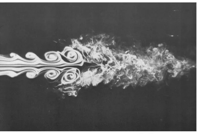
1.1 Vortex ring instability in a round jet at a Reynolds number of

about 13,000 . . . 2

1.2 U-shaped vortices formed by water boatman locomotion . . . 3

1.3 Vortex ‘steam’ ring shed from Mount Etna, Sicily, on 24th Febru-ary 2000 . . . 4

2.1 Shear layer instability as demonstrated by Rosenhead . . . 8

2.2 Velocities induced by singular and regularised particles . . . 9

2.3 Computational effort for velocity calculations vs. number of parti-cles, (*) Direct summation, (_¤) Fast multipole method, (+) VIC method on a cylindrical grid filled with 25% particles, (×) VIC method on a cylindrical grid filled with 65% particles, (_¥) VIC method on a cartesian grid filled with 100% particles . . . 11

2.4 Direct calculation of induced velocity . . . 15

2.5 Step 1 of PIC algorithm – Spread Γp . . . 15

2.6 Steps 2 & 3 of PIC algorithm – Solve, Convect . . . 17

3.1 Section of vortex tube showing vortex lines . . . 25

3.2 Section of vortex tube showing circulation Γ . . . 26

3.3 Section of vortex tube showing vortex strength α _{. . . .} ₂₇

3.4 Stretching and tilting of fluid element by ∇u . . . 28

3.5 Allowable vortex line configurations . . . 32

(9)

LIST OF FIGURES LIST OF FIGURES

4.1 Solution periodicity in x and y directions . . . 38

4.2 Introduction of errors through deformation of filaments . . . 45

4.3 Comparison of traditional to Cottet PIC . . . 47

4.4 (a) Magnitude of interpolation error vs. node spacing. (b) Magni-tude of mean error . . . 51

4.5 (a) Magnitude of finite difference error vs. node spacing. (b) Magnitude of mean error . . . 52

5.1 Video stills taken from experiment by Lim [1] of leapfrogging vortex rings . . . 55

5.2 Video stills taken from experiment by Lim [2] of obliquely colliding vortex rings . . . 56

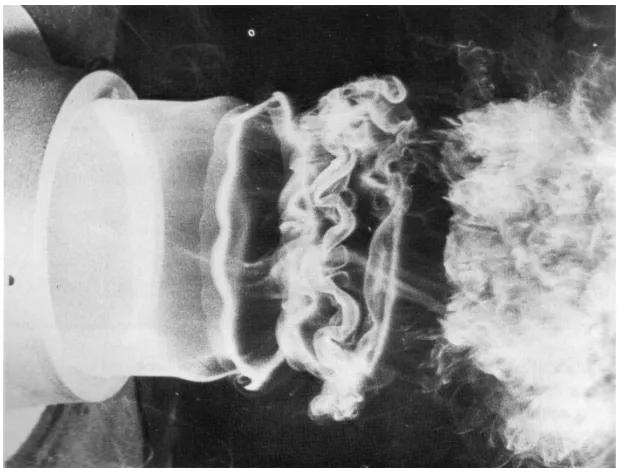
5.3 Vortex ring formation, visualised by dyed streaklines (D. Sallet, University of Maryland) . . . 57

5.4 Round jet instability: A jet at Reynolds number 10,000 devel-ops axisymmetric oscillations, rolls up into vortex rings, and then abruptly becomes turbulent. (Drubka & Nagib) . . . 57

5.5 Geometry of nozzle vortex-sheet model . . . 58

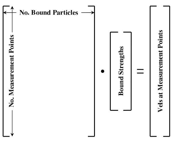
5.6 Equation set solved using least squares . . . 60

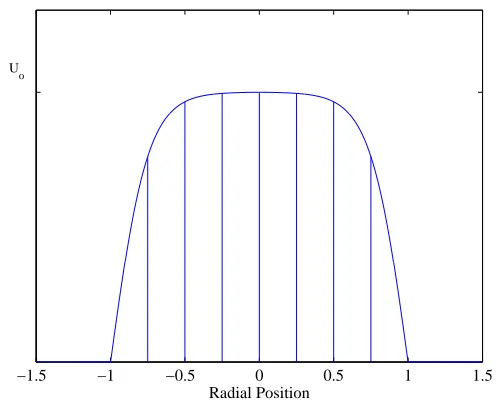
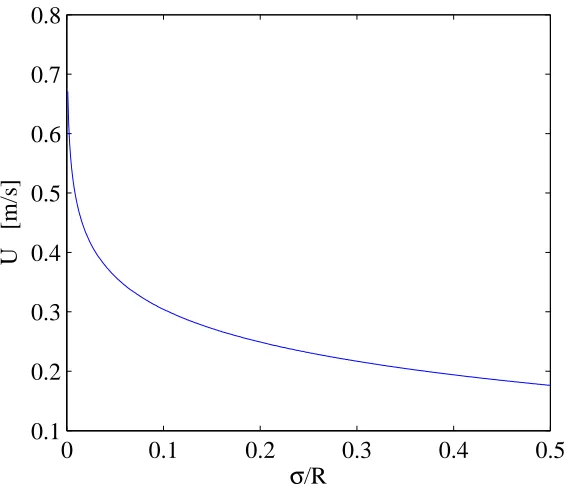
5.7 Spatial velocity profile, defined in equation 5.1 . . . 61

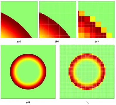
5.8 (a) Required vorticity profile at jet exit. (b) Direct discretisation 61 5.9 (a) Section of required vorticity profile at jet exit. (b) Subsampled vorticity field. (c) Summation of sub-samples at particle location. (d) Required vorticity profile at jet exit. (e) Discretisation using subsampling . . . 62

5.10 Isosurface of vorticity, (a) without and, (b) with subsampling at initialisation . . . 63

(10)

6.2 Application of azimuthal perturbation: k = 7, A = 0.1. Vorticity

vectors shown in red . . . 69

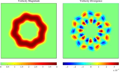
6.3 Initialisation divergence error: k = 8, A= 0.05, ∆ = 0.05 . . . 70

6.4 Problem geometry for oblique collision of vortex rings . . . 77

6.5 Obliquely colliding rings problem, Γ = 1, R = 1, S = 2.7, α = 15o_. _top _{Winckelmans & Leonard simulation.} _middle _Vorticity isosurface,|ω_|_{= 0}_._5. _bottom _{Scalar particles. . . .} ₇₈

6.6 Fig. 6.5 cont. . . 79

6.7 Fig. 6.5 cont. . . 80

6.8 Results from current study at T = 16.0 . . . 81

6.9 Comparison of enstrophy development with Winckelmans & Leonard [3] . . . 81

6.10 Number of particles in domain versus time. Minimum allowable strength = 5×104_{· |}_α_| max at t= 0 . . . 82

6.11 Diagram of Didden’s experiment [4], showing relevant terminology 82 6.12 Temporal velocity profiles, defined by equation 6.10 . . . 83

6.13 Vortex ring diameter vs. axial distance from tube edge. . . 83

6.14 Comparison of circulation shedding rate with results from Nitsche & Krasny, Didden and slug flow model . . . 84

6.15 Visual comparison between Didden’s experiment (top), Nitsche & Krasny’s numerical model (δ = 0.2) (middle) and current study (bottom) for vortex ring generation problem. . . 85

6.16 Fig. 6.15 cont. . . 86

6.17 Measured and theoretical linear impulse . . . 87

6.18 Measured and theoretical linear impulse . . . 87

6.19 Azimuthal vorticity contours . . . 88

6.20 Figure 6.19 cont. . . 89

6.21 Vorticity magnitude isosurfaces . . . 90

6.22 Figure 6.21 cont. . . 92

(11)

A.1 B-splines of increasing order used in interpolation . . . 94 A.3 Straight and rotated FD stencils . . . 97 A.2 Stencil of grid points for use in calculating ∇2_ω _(weights

(12)

List of Tables

2.1 Chronological summary of three-dimensional vortex simulations . 19

4.1 Steps in FFT of Poisson solver . . . 36 4.2 Options for periodic boundary condition (LPEROD) in Poisson

solver . . . 37

6.1 Normalised self-induced velocities for varying core radii, R = 1, Γ = 1 . . . 68

(13)

Nomenclature

xp Particle position vector

α_p _{Particle strength vector} ω _{Vorticity vector}

u Velocity vector Γ Circulation Ψ Stream function

∇u Velocity gradient tensor

S _{Rate-of-strain tensor} R _{Rotation tensor}

u−ω _{Velocity-vorticity formulation}

Ψ−ω _{Stream function-vorticity formulation} VIC Vortex In Cell

RHS RightHand Side BC Boundary Condition FFT Fast Fourier Transform

(14)

Chapter 1 Introduction

Computational fluid dynamics (CFD) has fast evolved from a mathematical cu-riosity to a standard tool in the analysis of fluid flows. It is defined as the numerical solution, by computational methods, of the governing equations which describe fluid flows. The attraction of CFD is that it offers a convenient means of understanding flows which can prove either too difficult or overly expensive for traditional experimental techniques. The sharp increase in computational power since CFD was first introduced has presented more and more opportunities to model flows previously analysed only in experiments.

However, this computational power has a finite upper limit, and so there will always be a place in CFD research for investigating novel techniques for solution of the governing equations, in the hope that they will offer improved performance over traditional approaches. Vortex methods are a family of techniques that fall into this category, and they have been investigated extensively since their first use by Rosenhead [5].

The class of vortex methods examined in the current study areParticle-In-Cell techniques. Basically, these techniques share a common feature with all vortex methods in that it is the development of the vorticity field which is examined, and this vorticity field is discretised onto a set of particles. These particles are then convected in a velocity field which is calculated on a fixed mesh. This hybrid

(15)

Introduction

approach ‘cherry-picks’ the best features of the Lagrangian and the Eulerian approach, to give a combined algorithm more efficiency and robust than the two in isolation. This will be discussed in more detail in chapter 2.

[image:15.595.168.478.262.499.2]

A common feature in all of the flows analysed herein is the presence of coherent vortex structures. Examples of such structures in engineering are the vortex ring structures in the potential core region of free jets, as illustrated in Fig. 1.1, or the trailing vortices from the wingtips of aircraft.

Figure 1.1: Vortex ring instability in a round jet at a Reynolds number of about 13,000

(16)

Introduction

[image:16.595.200.447.150.494.2]

generated by motion of its legs propels the insect forward. This motion is clearly illustrated in Fig. 1.2.

Figure 1.2: U-shaped vortices formed by water boatman locomotion

While the modelling of jets similar to that shown in Fig. 1.1 is the primary aim of this study, vortex rings are used extensively in this work to test various aspects of the model. Generation of these structures is most familiar as a measure of a smoker’s prowess, though similar structures have been witnessed in nature from the craters of volcanoes. Measuring up to 200m in diameter, a very clear example is shown in Fig. 1.3.

The modelling of jets like that shown in Fig. 1.1 is important for several reasons. Noise reduction from commercial aircraft is a huge area of research at present, as strict new environmental noise legislation requires drastic reductions

(17)

[image:17.595.169.477.105.323.2]

Introduction

Figure 1.3: Vortex ‘steam’ ring shed from Mount Etna, Sicily, on 24th February 2000

in all aspects of aircraft noise. On takeoff, jet noise is one of two dominant noise sources (the other is fan noise) and can generate noise levels over 90dB. Attempts to reduce this noise usually consist of modifying the shear layer structure in some way, either by shielding the central core with a lower speed jet (co-axial configuration) or by using modified exhaust nozzle shapes to break up the strong velocity gradients (e.g. scalloping). Modelling the effect of these modifications on the flow field is important to understand their effect on the resulting noise generated.

There are three main categories of CFD which have been applied to the prob-lem of jet flows. These are, in order of computational power required: Reynolds-averagedNavier-Stokes,Large-EddySimulation andDirectNumericalSimulation.

(18)

Introduction

modelling) being used increasingly frequently in the literature. The applicability of RANS is limited however, as no transient data is generated. A more recent development, Unsteady RANS, offers a means of recovering at least part of the turbulent data, as the unsteady term is retained in the usual RANS equations. However, a turbulence model is still required in the spatial discretisation, so it cannot fully resolve the turbulent data.

In LES only the large scales of the flow must be resolved, and asub-grid scale Reynolds stress is used to model their influence on the smaller, unresolved, scales. This increases greatly the Reynolds number which can be modelled, though large parallel computers are still required to perform calculations. Jets with Reynolds numbers of the order of ReD = 1.0×105 have been successfully modelling using

this approach [6].

In DNS, all scales of the turbulent flow must be resolved, which requires an extremely fine mesh, and therefore huge computational power, even for jets with Reynolds number of a few thousand.

A recently developed hybrid technique uses RANS at certain mesh and im-mersed boundaries and LES for the free field dynamics. This greatly reduces computational effort required, especially for complex geometries, such as scal-loped nozzles.

Understanding the fluid dynamics of jet flows is usually focussed on the be-haviour of coherent vortex structures in the flow, e.g. the reorientation from az-imuthal to streamwise vorticity and the ultimate breakdown of these structures to fully turbulent flow. Modifications to the nozzle geometry has a direct impact on these features, for example scalloping of the jet nozzle excites the stream-wise vorticity generation mechanism and accelerates the vortex breakdown. It is therefore an intuitive approach to use vortex elements as a basis in the modelling of such flows, as it is their behaviour that is of the most interest.

These vortex elements are discrete packets of vorticity, and it will be shown in later sections that by using these elements, or ‘particles’, it is only necessary

(19)

1.1. _{Objectives & Outline} _Introduction

to track their change in position and strength due to local gradients in velocity and vorticity in order to adequately represent the entire flow field.

1.1 Objectives & Outline

As a first step to solving a flow from a full-scale jet engine, the objective of this work is to develop a computationally inexpensive code, based on vortex methods. Parallel computing strategies are not considered, as the focus is on the underlying algorithm development. This requires a code that can solve for fully three-dimensional transient incompressible viscous flow on a single computer processor. A suite of algorithms is developed to deal with each aspect of the discretisation of the governing equations.

(20)

Chapter 2 Literature Review

2.1 Vortex Methods . . . 7

2.1.1 Viscous Diffusion . . . 10

2.1.2 Three Dimensions . . . 13

2.2 Particle In Cell . . . 14

2.2.1 Three dimensions . . . 17

2.1 Vortex Methods

Vortex methods for the study of fluid flows were initiated by L. Rosenhead in 1931 [5]. He used a small system of singular point vortices to represent an inviscid shear layer. When the particle locations were perturbed sinusoidally, the sheet rolled up, demontrating the Kelvin-Helmholtz instability. This behaviour is shown in the series of images, Fig. 2.1.

Rosenhead was only able to solve four time iterations however, as he had to perform all calculations by hand.

Subsequent work by other authors attempted to improve the accuracy of the same technique by performing their calculations on early computers, but quickly

(21)

2.1. _{Vortex Methods} _{Literature Review}

ran into trouble with very large induced velocities when two point vortices ap-proached too close to each other, due to the singular nature of their vorticity distribution.

0 1 2 3 4

Figure 2.1: Shear layer instability as demonstrated by Rosenhead

Vortex blobs, introduced by Chorin in [7], remove the singularity, either by directly modifying the velocity field or by replacing the Dirac delta function with a smooth vorticity distribution model. Chorin used the first approach and applied a cutoff function that limited the maximum possible velocity. Modern discrete vortex methods use the second approach; a wide variety of core models have been designed, (see [3] for an exhaustive list). Recent work has achieved excellent spatial resolution with this method, provided certain convergence criteria are observed [8]. The velocity fields induced by a singular particle, a Chorin-type particle, and a standard Gaussian core model vortex are plotted in Fig. 2.2.

(22)

Several techniques have been developed to reduce this cost. Purely Lagrangian approaches subdivide into two closely related techniques,treecode algorithms, [9], and fast multipole methods, [10]. The basic concept behind both of these tech-niques is the same–to subdivide the particle field into a hierarchy of clusters based on their spatial locations. Depending on two clusters’ separation, their effects on each other can be treated as single cluster-cluster interactions, or particle-cluster interactions.

In a treecode algorithm, the particles are divided into a nested set of groups and the O(N2_{) particleparticle interactions are replaced by a smaller number of} particlecluster interactions. The fast multipole method is more complex, requir-ing the use of spherical harmonics in three dimensions. The FMM also employs a more elaborate evaluation procedure in which the far-field multipole approxi-mation is modified at the local particle level. Both of these algorithms can lead to computations that scale linearly with the number of particles, O(N).

0 1 2 3 4 5 6

u θ

|r|/σ

Singular Chorin Lamb Vortex

∞

(2πσ)−1

Figure 2.2: Velocities induced by singular and regularised particles

(23)

The fast multipole method has been implemented successfully in 2D for com-putations involving millions of particles [8]. The treecode algorithm outperforms the fast multipole method in three-dimensional simulations, due to its simpler hierarchy interactions. An excellent example of its application is given in [11].

In the same year as Chorin’s seminal paper, Christiansen [12] sidestepped the O(N2_{) nature of the velocity calculation, while also avoiding the singularity} problem in a different way. He applied the recently developed particle-in-cell [PIC] [13] technique to fluid-flow problems using vortex methods.

Maintaining a singular vorticity distribution on the vortex particles, a fixed Eulerian grid is used to calculate their induced velocity field. Clearly, there can be no singular velocities as there is an implicit smoothing involved in reconstructing the vorticity field on the underlying grid. Fast Poisson solvers can be used for the velocity calculations, yielding computational performance ofO(MlogM), where M is the number of grid points. This technique is described in detail in§ 2.2, as it forms the basis of the work in this thesis.

As for the question of PIC efficiency versus pure Lagrangian techniques, this cannot be answered simply. The efficiency of both approaches is entirely depen-dent on the geometry of the problem being modelled. For example, a purely La-grangian approach will always outperform a PIC approach for modelling wingtip vortices or other highly compact elongated region of vorticity. For regions of distributed vorticity, the PIC approach is much faster. This is summarised math-ematically in [11] where the performance of both approaches is compared for different particle densities in the same domain.

Computational power required for several different computations in the liter-ature are summarised in Fig. 2.3.

2.1.1 Viscous Diffusion

(24)

method. Early techniques primarily modelled inviscid flows, as do most current vortex filament techniques. However, particle-based vortex methods offer a range of ways of accurately incorporating viscous effects into a simulation.

Viscosity tends to decrease gradients in the vorticity field, smoothing out peaks and increasing the overall support of the vorticity. While redistribution of particle strengths is the obvious approach to modelling this effect, altering particle locations can have a similiar effect, as seen in the random walk method.

Three separate approaches were examined in this study.

Random Walk Simplest means of modelling diffusion, requires large number of particles, unsuitable for 3D.

103 104 105 106 107

10−1

100

101

102

103

104

Number of Particles

CPU Time

Figure 2.3: Computational effort for velocity calculations vs. number of par-ticles, (*) Direct summation, (_¤) Fast multipole method, (+) VIC method on a cylindrical grid filled with 25% particles, (×) VIC method on a cylindrical grid

filled with 65% particles, (_¥) VIC method on a cartesian grid filled with 100% particles

(25)

Particle Strength Exchange Offers highest resolution, very computationally expensive

Mesh-based Limited resolution, very efficient.

Chorin was the first to use the random vortex method. This method is based on the fact that the probability of existence of a particle moving at random, like Brownian motion, is determined by the diffusion equation. The random walk added to the motion of the vortices reproduces the viscous diffusion in a statisti-cal sense. While this is a very attractive technique for its simplicity it does have its limitations. A huge number of particles is required to ensure accurate repre-sentation of the diffusion mechanism, which caused problems for early researchers using this technique. Chorin himself wrote “we do not expect valid solutions at low Re”, due to the coarseness of the solution when the magnitude of the random walk becomes comparable to the convective effect. More recent work, for example [14], has yielded very satisfactory results using this technique. In the cited work,

O(105_{) particles were used to model 2D flow over a cylinder in cross flow.} Unfortunately, applying a random walk to three-dimensional particles vio-lates Helmholtz’s law. This introduces a random divergence into the vorticity field, so while its efficiency wold be even more appreciated in a three-dimensional calculation, it is unsuitable for this application.

The Particle Strength Exchange technique is a newer, more advanced, algo-rithm. Developed in [15], it has largely superceded all other purely Lagrangian techniques. The concept of this technique is to replace the Laplacian diffusion operator by an integral one,

∇2ω₌_σ2X

q

(volpωhq −volqωhp)ησ(xhq −xhp) (2.1)

Where ησ is the core model function. While each particle only affects a small

(26)

form of multipole expansion for efficient solution.

The nature of the technique also places strong restrictions on particle core overlapping, usually required frequent remeshing to ensure this criteria is met. This can cause difficulty for problems involving immersed boundaries.

The third technique examined is made possible by the use of a fixed Eule-rian mesh in the particle-in-cell approach. The diffusion equation can be solved directly on the mesh, and the results can be spread onto the particles using the same interpolation functions as for the vorticity and velocity. This treatment of viscous diffusion is discussed in greater detail in §.4.3.

2.1.2 Three Dimensions

Extension of vortex methods to three dimensions is not trivial. The stretching term, ω_{· ∇}_u _{in the vorticity transport equation Eq. 3.21 no longer reduces to} zero, as is the case in two-dimensional flow, and must be modelled with very high accuracy, as it is now the dominant mechanism responsible for redistribution of the vorticity field. It is the treatment of this term that subdivides the two different approaches to this problem.

Vortexfilaments, introduced by Leonard, [16, 17, 18], directly apply Helmholtz’s law that vortex structures must move as material lines. All that is necessary to track the development of these structures is to track the movement of the repre-sentative material lines. The stretching term is accounted for by ensuring that the vorticity vectors lie everywhere tangent to the material lines.

There are two main drawbacks to use of this technique. For viscous flows, the vortex filaments no longer retain their identity. In fact there is no guarantee that viscosity will alter the circulation uniformly around the circumference of a vortex filament, and so the technique is invalidated. A further problem arises in the generation of vortex filaments from immersed boundaries, where the exact structure of the filaments shed from the surface must be known a priori. These factors greatly limit the technique’s applicability beyond idealised inviscid flows.

(27)

2.2. _{Particle In Cell} _{Literature Review}

Vortex particles, or vortons, or vortex sticks as they have been variously termed, were first used by Rehbach, [19, 20] for modelling three-dimensional vortex sheets. They are a direct extension of the classical two-dimensional vortex particle scheme, with the necessary additions to handle vortex stretching. De-tails of the treatment of this term are in §.4.2. The vortex particle technique has largely superseded vortex filaments, as models can incorporate both viscous diffusion and complex immersed boundaries.

2.2 Particle In Cell

The concept of classical particle-in-cell in the context of vortex methods is ex-plained here. Current developments involve higher order spatial interpolation and temporal integration, but the fundamental principal of the method has not changed.

The basic problem required to be solved by discrete vortex techniques is sketched in Fig. 2.4. A distributed group on particles, of numberN, each carrying circulation are used to represent a smooth vorticity field. The induced velocity at each particle location is calculated by summing the influence of every other particle in the field, so the number of calculations required is O(N2_{). Clearly,} computational power required becomes prohibitively expensive for even a modest number of particles.

(28)

• O(N2_{) calculations}

• Core model required

Figure 2.4: Direct calculation of induced velocity

The original vortex Particle-in-Cell technique as developed by Christiansen [12] is designed specifically to overcome these two drawbacks. The vortex par-ticle distribution is overlaid with a fixed Eulerian grid. Using some form of particle-mesh interpolation–in this instance a simple area-weighting–the particle circulations are spread onto the nodes of the fixed grid. The vorticity field can now be calculated by scaling the nodal circulations by the areas associated with each grid node. This step is illustrated in Fig. 2.5.

• Spread circulations Γp to

mesh

• Simple area weighting

• Scale by area to give ω_m

Figure 2.5: Step 1 of PIC algorithm – Spread Γp

(29)

Once the vorticity field has been reconstructed on the grid, a Poisson equation is solved to calculate the velocities at the mesh nodes. Christiansen uses a stream function-vorticity formulation (Ψ−ω_),

∇2Ψ =−ω

An advantage of this approach is that it is now only necessary to solve a sin-gle Poisson equation (In 3D this advantage does not apply). The two velocity components are calculated by differentiation of the stream function on the grid. However, this clearly reduces the order of continuity of the solution by one, which will limit the spatial resolution of the solution, making it necessary to have a high mesh density in locations of high strain.

An alternative approach to the stream function formulation is to use a velocity-vorticity formulation (u−ω_{). There is now a set of either 2 or 3 Poisson equations} to be solved, depending on the dimension of the system,

∇2u=∇ ×ω

(30)

• Solve Poisson equation

→ um

• Calculate particle veloci-tiesupusing previous

area-weighting

Figure 2.6: Steps 2 & 3 of PIC algorithm – Solve, Convect

To finish the calculation loop, the same interpolation procedure that was used for the circulation spreading is now used to calculate the velocity at each particle location as a function of the velocities just calculated at the neighbouring mesh nodes, (See Fig. 2.6).

2.2.1 Three dimensions

The first application of PIC-type techniques for calculation of three-dimensional flows was by Cou¨et et al, [21]. Using filaments rather than particles, discrete marker points are used to represent the vortex filaments, and these points are convected according to the induced velocity field. This field is calculated in an identical manner to Christiansen’s original PIC technique. Poisson solver calculations are performed in Fourier space to aid computational efficiency, a modification described in detail in § 4.1.1. The stretching term is dealt with by enforcing that point vorticity vectors remain tangent to the filaments, and by ensuring the vorticity magnitudes are altered according to the local stretch at the point locations.

The first attempt at actual three-dimensional particle-in-cell was by Brecht

(31)

& Ferrante for studies of inviscid buoyant bubbles [22][23]. Table.2.1 summarises major publications in the field to date.

(32)

2 .2 . P a r t ic l e In C e l l L it e ra t u re R e v ie w

Author(s) Year Re Simulations Vel. Calcs.

Rehbach 1978 inviscid Shed vortex sheet Direct

Cou¨et et al. 1981 inviscid CHECK PIC

Brecht & Ferrante 1989 invsicid Buoyant bubbles PIC

Knio & Ghoniem 1990 inviscid Perturbed vortex ring CHECK

Winckelmans & Leonard 1993 400, inviscid Colliding vortex rings Direct

Ould-Salihi et al. 2000 1400 Impinging vortex ring PIC

Liu & Doorly 2000 1000, inviscid Colliding vortex rings PIC

Walther & Koumoutsakos 2001 180, 230 Falling drop PIC

Ploumhans & Winckelmans 2002 300, 500, 1000 Impulsively started sphere Tree Code

Huberson & Voutsinas 2002 inviscid Shed vortex sheet PIC

Cottet & Poncet [24] 2004 300, 400 Impulsively started cylinder /

Impinging vortex ring

PIC

Table 2.1: Chronological summary of three-dimensional vortex simulations

(33)

Chapter 3 Fundamental Concepts

3.1 Lagrange vs. Euler . . . 20

3.2 Vorticity . . . 22

3.2.1 Points, Blobs, Sheets, Filamentsetc. . . 24 3.2.2 Circulation, Γ . . . 25

3.3 Velocity gradients . . . 27

3.4 Vorticity dynamics . . . 29

3.4.1 Helmholtz’s and Kelvin’s Laws . . . 31

3.1 Lagrange vs. Euler

(34)

3.1. _{Lagrange vs. Euler} _{Fundamental Concepts}

the basis for major commercial codes.

The second,Lagrangian, method follows the positions of fluid particles as they move in the fluid, flow information is now stored on the particles. The values of the various fluid properties at these particle locations are determined as they convect in the flow, and in this way the behaviour of the flow is captured.

Both techniques have inherent advantages and disadvantages. To solve for a field variable in a certain domain, an Eulerian approach superimposes a grid over the entire domain. The boundaries of this grid usually have to extend outwards quite substantially, in order to avoid spurious interactions between the flow and the grid boundaries. Lagrangian techniques on the other hand, need only ever place particles where they are required, so far fewer calculations are required.

Fortunately, several types of fast solvers have been developed for use on fixed grids, so this speed-up usually far outweighs the advantage of smaller solution set requirements in the Lagrangian approach. However, in situations where the distribution of the field property in question is very compact, (i.e. wing-tip vortices, free jets) this may not always be the case, as the majority of calculations in the Eulerian approach will be redundant. A quantitative comparison of this issue was illustrated in Fig. 2.3.

Most CFD techniques often require the ability to match computational point density to gradients of one or more of the flow properties being examined, both to ensure solution convergence and accuracy. An example of this requirement is the resolution of a turbulent boundary layer, where, due to the extremely high velocity gradients normal to the wall, very high mesh density is required for Eulerian velocity field calculations. This mesh refinement becomes extremely laborious, especially in three-dimensions, and also requires a reasonably accurate knowledge of the expected flow-field a priori.

With Lagrangian techniques, free particles are the computation points, and it is a trivial operation to alter their density to match the solution requirements. A further advantage is that the particles will largely follow the gradients of the

(35)

3.2. _Vorticity _{Fundamental Concepts}

flow in which they are convecting, giving a crude form of self-refinement.

3.2 Vorticity

The motion of a fluid is described by the velocity field u(x, t). The curl of the velocity field is called the vorticity, ω_(x_{, t}_{). In 3D cartesian coordinates,}

ω₌_{∇ ×}_u₌

          ∂w ∂y − ∂v ∂z ∂u ∂z − ∂w ∂x ∂v ∂x − ∂u ∂y           (3.1)

It follows from the definition that the vorticity is solenoidal, i.e. there cannot be divergence present in the vorticity field,

∇ ·ω _{= 0} _(3.2)

Physically, vorticity is a measure of the rotational characteristics of a flow. For a infinitesimal fluid element in that flow, its vorticity is twice its average angular velocity. The use of this property as the basis for a computational technique is obvious, and it is this link that is the starting point of all vortex methods.

A property related to the vorticity field in a similar way that kinetic energy is related to the velocity field is the enstrophy, E which is simply the square of the vorticity, ω _·ω_{. This property is used as a measure of the total vorticity} present in the flow, and the change in total enstrophy with time is an important diagnostic in analysing the amount of vortex stretching acting on the vorticity. This behaviour is described in more detail in A. A.3.

(36)

invariant, even with viscous effects present in the flow. The linear impulse is defined as

I ₌ 1 2

Z

x×ω_d_x _(3.3)

It is shown in Saffman [25] that this plays the part of momentum in unbounded flows, because

dI dt =

Z

F dx (3.4)

where F is the sum of the non-conservative external body forces. Clearly, if the right hand side is zero then there can be no change in the value of I _even when the flow is unsteady. Also, for jet flows, the value of I _{should increase} linearly as a function only of the jet velocity and nozzle area

Knowledge of the vorticity means that the velocity field is known implicitly, and vice versa. The vorticity field can be recovered from a velocity field simply from its definition Eq. 3.1. Calculation of the velocity field from a given vorticity distribution requires either the solution of the Biot-Savart law, or a Poisson equation in either velocity or stream-function form.

The exact form of the Biot-Savart law differs depending on the dimension of the problem,

u=

Z

K(x−y)×ω_(y)_d_y _(3.5)

K(z) =     

−₂1_πz/|z|2 _{in two dimensions} 1

4πz/|z|3 in three dimensions

(3.6)

In purely Lagrangian solvers, the Biot-Savart law is discretised to give a sum-mation equation for the velocities induced by a set of finite vortex particles. In particle-in-cell techniques, a Poisson equation is solved on the fixed grid in order to find the particle velocities.

(37)

3.2.1 Points, Blobs, Sheets, Filaments

etc.

It is relevant at this stage to give a brief summary of the terminology associated with various vortex structures. In two dimensions there are three main types,

Points Point vortices are singular distributions of vorticity, where the vorticity is represented by a Dirac Delta function

Blobs By convolving a point vortex with a smoothing function, the vorticity distribution is spread outwards, usually in the form of a Gaussian.

Sheets Vortex sheets are singular distributions along a line, as opposed to on a point.

In three dimensions the situation becomes more interesting.

Points Identical to singular particle in 2D, except vorticity now represented by a vector.

Blobs 2D smoothing functions can be extended to 3D, giving a natural equiva-lent.

Vortex line Just as a streamline is a curve which is always tangent to the ve-locity field, can define a vortex line as a curve which is always tangent to the local vorticity field.

Vortex tube The surface that is formed by all the vortex lines passing through some closed curve in space. A schematic of a vortex tube made up of several vortex lines is shown in Fig. 3.1.

Vortex ring If a vortex tube forms a closed loop, it is termed a vortex ring. Vortex filament If the cross-section of a vortex tube is made infinitesimally

(38)

Figure 3.1: Section of vortex tube showing vortex lines

3.2.2 Circulation,

Γ

A scalar property of importance in the description of vortex flows is the circula-tion, Γ. Whereas the vorticity describes rotation at a point, circulation describes

the total rotation over a defined region. It can be defined in two ways. The first is as an area integral over a given vorticity distribution

Γ =

Z

A

ω_·_d_A _(3.7)

From application of Stokes’ theorem, circulation can also be defined as the line integral of velocity around a closed curve enclosing the region of vorticity

Γ =

I

C

u·ds (3.8)

(39)

Sign convection for vorticity and circulation obeys the right-hand rule, i.e. anticlockwise circulation is positive.

A section of vortex tube, shown in Fig. 3.2, is used to demonstrate the eval-uation of the circulation of a finite region of vorticity. The circulation cannot change along the length of the tube, from Helmholtz’s first law, (see §3.4.1).

Figure 3.2: Section of vortex tube showing circulation Γ

Another property, related to the circulation, is the vortex strength, α_{. It has} units of vorticity×volume.

α=

Z

V

ω_·_d_V _(3.9)

If a vorticity-carrying fluid element is thought of as a small section of a vortex tube, as shown in Fig. 3.3, it can also be defined as circulation×length–where the length is of the section of tube the element represents.

(40)

3.3. _{Velocity gradients} _{Fundamental Concepts}

Figure 3.3: Section of vortex tube showing vortex strengthα

3.3 Velocity gradients

Spatial velocity gradients are important for two reasons. Firstly, they govern the behaviour of the non-linear stretching term in the momentum equation. Secondly, they give a physical description of the deformation of the particles behaving as fluid elements.

The velocity gradient tensor, present in the stretching term in Eq. 3.21, can be written in full as

∇u=

           ∂u ∂x ∂u ∂y ∂u ∂z ∂v ∂x ∂v ∂y ∂v ∂z ∂w ∂x ∂w ∂y ∂w ∂z            (3.10)

The effect of each component on an initially cubic fluid element is illustrated in Fig. 3.4.

(41)

3.3. _{Velocity gradients} _{Fundamental Concepts}

Any second-order tensor can be decomposed into two separate tensors, one symmetric and the other skew-symmetric, using the identity

∇u= 1

2(∇u+∇u

T_{) +} 1

2(∇u− ∇u

T₎ _(3.11)

These two new tensors, widely used in fluid dynamics, are identified as the rate-of-strain and rotation tensors.

S ₌ 1

2(∇u+∇u

T₎ _{Rate of strain tensor}

R ₌ 1

2(∇u− ∇u

T₎ _{Rotation tensor} _(3.12)

(3.13)

(42)

3.4. _{Vorticity dynamics} _{Fundamental Concepts}

Using the definition of vorticity, R_{can be rewritten as}

R₌     

0 −ωz ωy

ωz 0 −ωx

−ωy ωx 0

     (3.14)

In calculation of the stretching term in Eq. 3.21, the product of this tensor with the vorticity vector is identically zero, therefore only the rate-of-strain tensor contributes to changes in the vorticity field through stretching.

When investigating the contribution fromS_{, it is useful to further subdivide it}

into two further tensors, one containing the diagonal components, and the other containing just the off-diagonal components.

S₌       ∂u

∂x 0 0

0 ∂v

∂y 0

0 0 ∂w

∂z       +1 2        0 ∂u ∂y + ∂v ∂x ∂u ∂z + ∂w ∂x ∂u ∂y + ∂v ∂x 0 ∂v ∂z + ∂w ∂y ∂u ∂z + ∂w ∂x ∂v ∂z + ∂w ∂y 0        (3.15)

As the flow is incompressible, the trace of the first tensor is zero. The three terms in this tensor correspond to stretching of the fluid elements in each of the three directions, as shown on the diagonal in Fig. 3.4. A positive value of one of these terms will cause an amplification of the existing vorticity component in the same direction when calculating the stretching term.

The second tensor contains information on how the fluid elements are being sheared by the local velocity gradients. There are only three independent terms, each modifying two of the vorticity components in calculation of the stretching term.

3.4 Vorticity dynamics

The incompressible Navier-Stokes equations are the starting point for the deriva-tion of the equaderiva-tions governing the vorticity dynamics.

(43)

∂u

∂t +u· ∇u = − 1

ρ∇p+ν∇

2_u _(3.16)

∇ ·u = 0 (3.17)

Whereu(x, t) is the velocity field,ω_(x_{, t}_{) is the vorticity field,}_p_{is the pressure,} ρ the density and ν is the kinematic viscosity.

The problem with using this set of equations as the basis for a computational technique is that it is necessary to solve for both the pressure and velocity com-ponents at every time step. As this is a nonlinear system, this requires iteration at every time-step to achieve the solution, with strict convergence criteria.

The vorticity transport equation is derived by rewriting Eq. 3.16 as,

∂u

∂t +ω×u=−∇( p ρ +

u·u

2 ) +ν∇

2_u _(3.18)

And then taking the curl of the resulting equation.

∂ω

∂t +∇ ×(ω×u) = ν∇

2_ω _(3.19)

The nonlinear term can be replaced using the identity

∇ ×(ω_×_{u) =} ₋_(u_·∇₎ω_{+ (}ω_·∇_)u _(3.20) Note that this identity only holds if ∇ ·u = 0 and ∇ ·ω _{= 0. While this} does implicitly incorporate the continuity equation into the vorticity transport equation, it will be shown in§4.5 that the vorticity field represented by a discrete set of particles cannot be guaranteed to remain divergence free for all times.

The vorticity transport equation can now be written in the familiar form,

∂ω

∂t + u· ∇ω = ω· ∇u + ν∇

(44)

Rate of change of ω

Convection Stretching Viscous diffusion

The discretisation of the three transport terms in Eq. 3.21, convection, stretch-ing and diffusion is described in § 4.1–§ 4.3.

3.4.1 Helmholtz’s and Kelvin’s Laws

Work published by Hermann von Helmholtz (1821-1894) in 1858, and by William Thomson, later Lord Kelvin (1824-1907) in 1869 initiated the mathematical study of vortex motion. They produced a set of laws that govern the behaviour of vorticity-carrying regions in a flow.

It is worth referring back to the diagram of the vortex tube in Fig. 3.1 in the previous section, as these laws are most readily explained in relation to such a structure.

Helmholtz’s first law states that, for inviscid flows, the substantive derivative of the circulation must always be equal to zero.

DΓ

Dt = 0 (3.22)

The substantive, or material, derivative is used to describe time rates of change in a Lagrangian frame, as it accounts for both standard variations in time, and also variations due to convection (D/Dt =∂/∂t+u· ∇).

A consequence of this law mean that fluid elements that at any instant lie inside a vortex tube will remain within the tube, independent of velocity gradients acting on the tube. A useful application of this law is that vortex filaments can be tracked through a velocity field by simply monitoring the material line corresponding to the initial filament centreline.

The inverse of this law means that any particle initially free of vorticity must remain irrotational for all consequent times.

(45)

Helmholtz’s second law states that the circulation of a vortex tube must be the same at all cross sections. Therefore, if the tube narrows due to local velocity gradients, the vorticity must increase.

This law also restricts the possible configurations of vortex lines and tubes. These structures must be stretch to infinity, end at a boundary, or form a closed loop. These three allowable configurations are shown in Fig. 3.5.

Kelvin’s law extends Helmholtz’s first law to include the effect of viscosity. For the circulation of a vortex tube in a viscous flow,

DΓ Dt =ν

Z

L

(∇2u)·dr (3.23)

Clearly, for inviscid flow, the RHS of Eq. 3.23 is zero, thus reducing to Helmholtz’s first law.

An interesting aside in Helmholtz’s publication was one of the first descriptions of leapfrogging vortex rings. He described his conclusions regarding two circular vortex rings with a common axis of symmetry as follows,

If they both have the same direction of rotation they will proceed in the

same sense, and the ring in front will enlarge itself and move slower,

while the second one will shrink and move faster, if the velocities of

(46)

translation are not too different, the second will finally reach the first

and pass through it. Then the same game will be repeated with the

other ring, so the rings will pass alternately one through the other.

An attempt at modelling this phenomenon is described in § 6.3. It is quite difficult to model the ‘game’ for long enough to capture the pass of the second ring back through the first ring, as this requires to maintain a near-inviscid flow regime for a relatively long simulation time. However, as will be demonstrated later, some diffusion is necessary to maintain solution stability.

It is not just numerical models that have problems with this flow however, as to date there has only been one successful experimental study of this ‘double-jump’ published [1].

(47)

Chapter 4 Numerical Modelling

4.1 Convection . . . 35

4.1.1 Poisson Solver . . . 35

4.2 Stretching term . . . 39

4.2.1 Analytical solution . . . 41

4.3 Diffusion . . . 41

4.4 Temporal Discretisation . . . 42

4.5 Vorticity Divergence . . . 43

4.5.1 Regularisation . . . 46

4.6 Error Analysis . . . 49

4.6.1 Interpolation . . . 49

4.6.2 Finite Difference . . . 50

4.6.3 Conclusion . . . 50

(48)

vor-4.1. _Convection _{Numerical Modelling}

ticity transport equation Eq. 3.21. In each time step, the vortex particles are convected with their local velocities, and their strengths are modified to account for stretching and diffusion. All field calculations are performed on the fixed Eu-lerian grid, and this information is transferred to the particles in order to advance the solution in time.

§ 4.1 deals with treatment of the convection term in the vorticity transport equation, and the tools required to model this term. §4.2 deals with the stretching term, § 4.3 with viscous diffusion. § 4.4 describes how the solution is advanced in time. § 4.5 discusses the problem of vorticity divergence related to three dimensional vortex particle methods, and finally § 4.6 gives a brief discussion of errors arising in calculation of each of the terms.

4.1 Convection

The use of vortex methods to represent the convection term in the vorticity transport equation is made possible by Kelvin’s theorem. This states that the circulation contained in a Lagrangian fluid element is conserved, provided that the flow is inviscid and there are no external forces. Therefore, the temporal development of a set of marker particles carrying concentrated vortex strength, equivalent to an initial vorticity field, can be used to represent the actual fluid dynamics. The convection term (u·∇)ω_{in Eq. 3.21 is thus not treated explicitly,} as it is absorbed into the Lagrangian material derivative on the particles.

4.1.1 Poisson Solver

The velocity field is calculated from the vorticity field using a system of Poisson equations

∇2_u₌_{−∇ ×}_ω _(4.1)

This equation set is derived by appling the curl operator to the vorticity

(49)

4.1. _Convection _{Numerical Modelling}

definition Eq. 3.1, and using the vector identity

∇ ×(∇ ×u) =∇(∇·u)− ∇2u (4.2) Use of the incompressibility constraint on the velocity field, (∇·u= 0) is also required.

There are several approaches available for solution of this equation set. The simplest of these is finite difference on a regular structured mesh, where a standard set of stencils are used to calculate the required gradients in equationeq:Poisson, and a set of linear equations is solved. Fast Fourier transforms can be used to reduce the computational cost of this approach from O(M3) to O(M2logM), where M is the number of mesh nodes.

More advanced techniques use coordinate mapping on the initially regular grid to provide finer mesh density in areas of high spatial gradients, or an entirely unstructured mesh is used. Clearly these approaches are much more computa-tionally demanding that the optimised FFT solver using the regular mesh, so it was decided to use the simplest solver in the current study. Another factor in this decision was that development of a fast Poisson solver was outside the scope of this work, and there are several open-source FFT solver codes available which can solve the specified equation set. fishpack[26] is used in this instance. Using the RHS as input, the following steps are performed.

1 Discrete Fourier Transform in x direction 2 Discrete Fourier Transform in y direction 3 Tridiagonal Solve in z direction

4 Inverse Transform in y direction 5 Inverse Transform in x direction

(50)

The following system of linear equations is solved by Fishpack.

C₁_·_(x_i−₁_,j,k₋_2x_i,j,k₊_x_i₊₁_,j,k₎₊ C₂_·_(x_i,j−₁_,k ₋_2x_i,j,k₊_x_i,j₊₁_,k₎₊

A(k)·xi,j,k−1+B(k)·xi,j,k+C(k)·xi,j,k+1 =F(i, j, k)

fori= 1. . . L, j = 1. . . M, k = 1. . . N (4.3)

where L, M and N are the number of grid nodes in thex, y and z directions respectively.

This represents a standard second-order centered finite difference of the Lapla-cian operator. The right hand side (i.e. the source term) of Eq. 4.3 is generated using the 4th-order finite difference stencils derived in A.2.

A limitation of the FFT approach is that some form of periodicity must be assumed in thexandydirections. The full set of options for the x- and y-direction periodicity boundary conditions are listed in table 4.2.

Periodic Options

0 x0 =xL xL+1=x1 1 x0 = 0 xL+1= 0 2 x0 = 0 xL+1=xL−1 3 x0 =x2 xL+1=xL−1 4 x0 =x2 xL+1= 0

Table 4.2: Options for periodic boundary condition (LPEROD) in Poisson solver

(51)

Analysis of the effect of each of these periodicity constraints of the calculated velocity field showed that case 0 had the least influence on the flow field. So for the x direction,

x(0, j, k) = x(L, j, k)

x(L+ 1, j, k) = x(1, j, k) (4.4)

and similarly for the y direction. The exact form of this periodicity is shown in Fig. 4.1.1.

Figure 4.1: Solution periodicity inx and y directions

There is no such periodicity restriction in the z direction, so any boundary conditions can be applied. This allows convection of vorticity into and out of the domain–an obvious requirement in the simulation of free jets.

(52)

4.2. _{Stretching term} _{Numerical Modelling}

convect out of the domain without any spurious feedback on the upstream flow. The following expression is used to ’decay’ the vorticity at the outflow

∂ω ∂t =C

∂ω

∂z (4.5)

This is the convective outflow boundary condition used widely in large eddy simulations. The value used for C _{is the local convection velocity, although it}

has been found that the effect on upstream vorticity is largely insensitive to choice of this value. Orlandi [27] uses a constant value of 0.6 of the normalised characteristic velocity, and solution insensitivity was again reported.

While all calculations in this solver are performed in single precision (i.e. 32 bit), it was established in analysis of error magnitudes that errors induced from this truncation were negligible in comparison to other errors (see § 4.6).

4.2 Stretching term

The stretching term in the vorticity transport equation causes local intensification and reorientation of the vorticity vector, governed by shearing forces acting on the vorticity field. This effect is not present in two-dimensional flows and is challenging to accurately model.

Particle strengths are modified according to the local discretisation of the stretching term (ω_·∇_{)u. The velocity gradient tensor} _∇_u((_x₎_p _{is evaluated on} the grid using finite differences. This tensor is then interpolated on to the particle locations using the standard B-spline interpolation (see§A.1). Particle vorticities can now be updated, as in a grid-free vortex method, by solving

∂ω

∂t = [∇u((x)p][ωp] (4.6) where ω_p _{is the vorticity at a particle location. High-order finite difference} stencils are used throughout, in an effort to avoid numerical error and numerical dissipative effects.

(53)

4.2. _{Stretching term} _{Numerical Modelling}

Another possibility which was investigated, derived by Cottet in [28], is based on the conservative form div(ω _:_{u) of the stretching term. The idea is to multiply} grid values of vorticity and velocity. The tensorωiuj is then differentiated on the

grid, and its divergence is finally interpolated on the particles to update their circulations. This last option has the advantage of being conservative at the grid level, even when the vorticity field is not exactly divergence-free. However, the classical formulation where the velocity gradient tensor is spread directly on to the particles was considered a simpler approach and is used throughout in calculation of the stretching term.

A major advantage of the u− ω _{formulation of the Poisson equation over} the Ψ−ω _{form becomes apparent here. If the stream-function were solved on} the grid, it would have to be differentiated once to calculate velocities, and a second time to calculate the velocity gradient tensor. However, if the velocity field is calculated directly by the Poisson solver using Eq. 4.1, only one level of differentiation is required to extract the required gradients, leading to a higher level of accuracy.

(54)

4.3. _Diffusion _{Numerical Modelling}

4.2.1 Analytical solution

An analytical expression for stretching term is derived in [29] for three-dimensional particles with core models,

d dtα

p ₌₋X

q

1 σ3

·

g(ρ) ρ3 α

p_×_αq₊ 1

σ2_ρ d dρ

µ

g(ρ) ρ3

¶

(αp_·_(xp₋_xq_))((xp₋_xq₎_×αq₎

¸

(4.7) where ρ = |xp ₋_xq_|_/σ _{is the distance between particles normalised by core}

width.

The case of singular vortex particles is derived by setting g(ρ) = 1 and 1

ρ d dρ(

g(ρ)

ρ3 ) =

−3

ρ5. The term q = p must also be excluded from the summation. Eq. 4.7 now becomes,

d dtα

p ₌ q6=p

X

q

3

|xp₋_xq_|5

¡_αp_·_(xp₋_xq₎¢¡

(xp−xq)×αq¢

− 1

|xp ₋_xq_|3α

p_×_αq _(4.8)

This expression is used in calculation of the error introduced in the mesh-based calculation of the stretching term.

4.3 Diffusion

As outlined in the literature review, it is very important to accurately model vis-cous effects in real-world flows. While several approaches were introduced, it was found that mesh-based evaluation of the viscous diffusion performed adequately for the flows of interest in this work, and was also much less computationally expensive than the particle strength exchange technique.

Calculation of the viscous diffusion requires evaluation of the Laplacian in Eq. 3.21. Peaks in the vorticity field will have a high value of the Laplacian, and so viscosity will have the highest effect on such regions.

The Particle Strength Exchange technique replaces the Laplacian with an in-tegral operator, not requiring regular particle spacing. The problem now becomes

(55)

4.4. _{Temporal Discretisation} _{Numerical Modelling}

O(N2_{), so requires some form of multipole expansion, in order to achieve some} level of computational efficiency.

Fortunately, where a fixed grid is used, ∇2_ω _{can be solved directly on the} grid using finite differences. The result can then be spread directly back onto the particles using the standard interpolation technique, and the particle strengths modified accordingly.

Clearly, the spatial resolution of the technique is limited by the mesh resolu-tion, and the scheme does not implicitly conserve circulation. However, simula-tions using this technique, coupled with frequent regridding, maintain circulation sufficiently well for this shortcoming not to be noticeable.

For high Reynolds number flows, it is only necessary to calculate the viscous diffusion term at integer multiples of the time-step. This is because, in term of overall effect on circulation magnitude, it has a minor effect in comparison to the stretching term.

4.4 Temporal Discretisation

In order to advance the solution in time, the convection and stretching term are coupled over several steps of a Runge-Kutta time-stepping algorithm.

(56)

4.5. _{Vorticity Divergence} _{Numerical Modelling}

q1 = ∆t·u(x0)−6e3 x₁ = x₀+1

3q1 q2 = ∆t·u(x1)−

10 3 e1−

5 9q1 x2 = x1+

15 16q2 q3 = ∆t·u(x2)−

15 8 e2−

153 128q2 x3 = x2+

8

15q3 (4.9)

Where ei are round-off errors, defined as,

e1 = (x1−x0)− 1 3q1 e2 = (x2−x1)−

15 16q2 e3 = (x3−x2)−

8

15eq3 (4.10)

The two memory registers are used to storexandq, though the algorithm can be modified to store x and u, an approach more suited to memory requirements of other subroutines.

4.5 Vorticity Divergence

The problem with three-dimensional particle methods is that they are not in-herently stable. This means that as a simulation is run, some form of error accumulates, usually leading to unphysical velocities, which eventually become singular. The errors are apparent in divergence present in the particle vorticity field.

Where the stretching term introduces strong local vorticity intensification, this leads to rapid distortion of the particle field. Regular redistribution of the particle strengths is thus required to maintain a smooth solution field. This

(57)

regridding is achieved using the same interpolation function as used to trasnfer data to and from the mesh to the particles. A full description of this function is given in § A.1.

A meaningful physical interpretation of this error is illustrated in Fig. 4.2. This shows a vortex filament before and after deformation due to velocity gradi-ents. Helmholtz’s laws state that the circulation must remain constant about the circumference of the filament, and that vorticity vectors must remain tangent to the filament for all times. So where the filament is stretched, the vorticity vector increases in magnitude, and where it is distorted, the vorticity vector changes its orientation accordingly to remain tangent to the filament.

This reorientation and amplification is dealt with implicitly in vortex filament techniques. Using Helmholtz’s second law, A filament can be represented by a spline or set of line segments, which are defined by a set of marker points. The vorticity carried by the marker points is altered depending on the reshaping of the lines on which they lie, an exact analogy of the physical situation.

In the Particle-in-Cell approach this filament is now represented by a set of independent particles carrying vortex strengths. The only effect these particles have on each other is through their induced velocities, there is no longer any geometric constraints. Because of this freedom, the particle strength vector is no longer constrained in any way by the underlying filament it is supposed to represent. Instead, its strength is altered according to the local velocity gradients, through the stretching term [∇u][ω_{]. The hope is that this alteration will mimic} the change in the filament.

So, what happens when there is an error in this stretching term? The effect of any errors is shown in the magnified section in Fig. 4.2. Blue vectors represent a solution by vortex filaments. Clearly, the magnitudes and orientation of these vectors change according to the deformation of the filament.

(58)

Figure 4.2: Introduction of errors through deformation of filaments

so violating the second law. It seems the largest source of error is in the off-diagonal terms in the velocity gradient tensor, as these are solely responsible for reorientation of the strength vector.

The vorticity field associated with a three-dimensional vortex particle tech-nique cannot be guaranteed to remain divergence free for all times. Theoretically, this represents a major problem, as a basis which is not divergence free,ω_p_(x_{, t}₎ is being used to represent a vector field that is required to be divergence free for all times, according to Helmholtz’s Laws. The particle method is only solv-ing what it sees in accordance with its particular discretisation of the vorticity transport equation Eq. 3.21 and its representation of the initial vorticity field, which, depending on the coarseness of the solution, can differ greatly form the actual physics. If this difference is allowed to develop unchecked, the solution can become a very poor representation of the real vorticity field, and may eventually become unstable. This fact is in opposition with two-dimensional singular vortex particles (i.e. point vortices) for which the particle vorticity field is

(59)

tionally divergence free, and is a serious obstacle to the validity of finitely many singular particles as a model for the solution of the three-dimensional vorticity equation.

In practice, fortunately, if this divergence is kept to a minimum, by careful solution of the stretching term and by regular reallocation of the vorticity onto a regular particle distribution, its effect on the solution can be reduced substan-tially. It is also critical to minimise divergence in the initial vorticity present in the flow, and any vorticity introduced at later times. So, in order to main-tain regularity of solution for long runs, some technique is required to remove this divergence from the vorticity field, while maintaining the correct flow field information. Such techniques are discussed in the next section §4.5.1.

4.5.1 Regularisation

One of the first attempts at vorticity divergence removal was introduced in [31] for a purely Lagrangian technique. At every time-step the particle strength vectors are modified using the filtering

αnew

p = (1−C)αoldp +C

∇ ×u(xp)

|∇ ×u(xp)|

|αold

p | (4.11)

where ∇ ×u(xp) is the true local vorticity field and where C is a relaxation

factor. Physically, this scheme acts as a ’spring’ that tries to maintain the particle strength vector aligned with the true vorticity vector. This is a very simple technique as no system of linear equations involving other locations needs to be solved.

However, this technique was developed, and proven satisfactory, in the context of purely Lagrangian techniques, and so does not account for extra errors involved in interpolating data back and forth from the grid.

Three dimensional vortex particle in cell technique