Journal of Criminal Law and Criminology
Volume 74
Issue 4
Fall
Article 19
Fall 1983
Improving the Analysis and Presentation of Data
on Case Processing Time
David W. Neubauer
Follow this and additional works at:
https://scholarlycommons.law.northwestern.edu/jclc
Part of the
Criminal Law Commons,
Criminology Commons, and the
Criminology and Criminal
Justice Commons
This Criminology is brought to you for free and open access by Northwestern University School of Law Scholarly Commons. It has been accepted for inclusion in Journal of Criminal Law and Criminology by an authorized editor of Northwestern University School of Law Scholarly Commons.
Recommended Citation
Copyright 0 1983 by Northwestern University School of Law Pftnfed in US.A.
IMPROVING THE ANALYSIS AND
PRESENTATION OF DATA ON CASE
PROCESSING TIME
DAVID W. NEUBAUER*
I. INTRODUCTION
Delay is one of the most pressing problems facing the American judicial system. Several prestigious national commissions have identi-fied delay as a critical problem.' In addition to the constitutional guar-antee of a speedy trial,2 federal and state legislatures have passed speedy-trial bills mandating that criminal defendants be processed within a set period of time.3 Advocates of judicial reform point to bur-densome caseloads and excessive delay as direct or indirect rationales for their proposals.4
The general public is similarly dissatisfied with slow and inefficient justice. Over fifty percent of the respondents in a survey conducted by the Yankelovich, Skelly, and White polling organization rated the effi-ciency of the courts as a "serious" or "very serious" social problem.5 Dissatisfaction and complaints, however, have far surpassed systematic
* Chairman & Professor, Political Science Dep't, University of New Orleans; Ph.D.,
Political Science, University of Illinois, 1971; M.A., Political Science, University of Illinois, 1968; A.B., Augustana (Illinois), 1966.
1 AMERICAN BAR ASSOCIATION PROJECT ON MINIMUM STANDARDS FOR CRIMINAL JUSTICE, STANDARDS RELATING TO SPEEDY TRIAL (1968); NATIONAL ADVISORY COMMIS-SION ON CRIMINAL JUSTICE STANDARDS AND GOALS, COURTS (1973) [hereinafter cited as NATIONAL ADVISORY COMMISSION]; TASK FORCE ON THE ADMINISTRATION OF JUSTICE, THE PRESIDENT'S COMMISSION ON LAW ENFORCEMENT AND ADMINISTRATION OF JUSTICE, THE COURTS (1967) [hereinafter cited as PRESIDENT'S COMMISSION].
2 U.S. CONST. amend. VI.
3 Speedy Trial Act of 1974, 18 U.S.C. §§ 3161-74 (1979); R. MISNER, SPEEDY TRIAL: FEDERAL AND STATE PRACTICE (1983); B. FORT, J. MCCULLOUGH, B. HOEL, J. MAIRS, J. SIMONITSCH, C. CLARK, P. HEENAN & L. CATr, SPEEDY TRIAL (1978); R. NIMMER, THE NATURE OF SYSTEM CHANGE 73-75 (1978); Misner, Delay, Documentation and the Speedy Trial
Act, 70 J. CRIM. L. & CRIMINOLOGY 214 (1979); Poulos & Coleman, Speedy Trial, Slow Imple-mentation The ABA Standards in Search of a Statehouse, 28 HASTINGS LJ. 357 (1976).
4 M. FEELEY, THE PROCESS IS THE PUNISHMENT: HANDLING CASES IN A LOWER CRIM-INAL COURT (1979); Nardulli, The Caseload Controversy and the Study of Criminal Courts, 70 J. CRIM. L. & CRIMINOLOGY 89 (1979).
5 Yankelovich, Skelly & White, Inc., Highlights of a National Surve of the General Public,
Judges, Lawyers, and Communi Leaders, THE PUBLIC IMAGE OF COURTS 1, 19 (1979).
DAVID W NEUBA UER
research on the subject. While the notion of "justice delayed is justice denied" is central to our system of government, it is only within the last several decades that empirical research has been brought to bear on this issue.6
The threshold problem faced by researchers is to develop a concep-tual definition of "delay" that can be measured.7 The prime utility of the term "delay" lies in calling attention to the problem area. Several major ambiguities, however, make the term "delay" inappropriate for research purposes.
In a general sense, the term "delay" connotes abnormal or unac-ceptable time lapses in the processing of cases. However, the inherent subjectivity of the term becomes apparent when we try to define "un-necessary delay." The total time that a case is on the court's docket may consist of acceptable (normal) time plus unacceptable (abnormal) time.8 In turn, many empirical measures of "delay" are measures of total time, that is, normal and abnormal time mixed together. Given that the term "delay" is typically used pejoratively to suggest unnecessary time, we need to keep in mind that not all case processing time is unnecessary.9 Yet it is difficult to determine what "normal time" for case disposition should be.10 Further, one must be mindful of varied and subjective local definitions. What is considered an old case in one community may be
viewed in another as merely ripe for disposition.'"
6 T. CHURCH, J. LEE, T. TAN, A. CARLSON & V. MCCONNEL, PRETRIAL DELAY: A REVIEW AND BIBLIOGRAPHY (1978).
7 Church, The "Old and the New" Conventional Wisdom of Court Delay, 7 JUST. Sys. J. 395
(1982).
8 R. NIMMER, supra note 3, at 72.
9 Luskin, Building A Theor, of Case Processing Tine, 62 JUDICATURE 114 (1978).
10 The reform literature discusses normal time and delay in reference to an ideal time
frame. R. NIMMER, supra note 3, at 72-73. A time interval cannot be considered normal or abnormal until such judgments are made. There is no consensus, though, about what this ideal time frame should be. The National Advisory Commission recommended 60 days from arrest to the start of trial of a felony prosecution. NATIONAL ADVISORY COMMISSION, supra
note 1, at 65. The earlier President's Commission specified a maximum of 81 days for the same events. PRESIDENT'S COMMISSION, supra note 1, at 86-87. The Federal Speedy Trial
Act mandates approximately 100 days. Speedy Trial Act of 1974, 18 U.S.C. § 1361 (1979). Other commissions, groups, and state speedy-trial laws have suggested time frames varying from six months to two years. JUDICIAL ADMINSTRATION: TEXT AND READING 15 (R. Wheeler & H. Whitcomb eds. 1977) [hereinafter cited as JUDICIAL ADMINISTRATION]. These varying and conflicting attempts to specify a maximally desirable time for disposing of a criminal case are largely abstract efforts. They are not grounded in a working knowledge of the dynamics of the court process. Moreover, they provide no linkages between the advan-tages to be derived from speeding up the dockets and the specific time frames. The President's Commission, for instance, acknowledged that its recommendations were the product of con-secutive, arbitrary choices. PRESIDENT'S COMMISSION, supra note 1, at 84.
11 A key dimension of a "local legal culture" is the local expectation about how long is too long for case dispositions. T. CHURCH, A. CARLSON, J. LEE & T. TAN, JUSTICE DELAYED 54 (1978) [hereinafter cited as T. CHURCH].
Recognition of these ambiguities has prompted researchers to adopt a more objective and measureable concept-case processing time.12 Case processing time is an objective measure of how long cases take from start to finish.
After adopting the proper definitional framework, secondary problems arise in using the concept of case processing time to generate empirical measures. The purpose of this Research Note is to examine some important conceptual, measurement, and analytical problems that arise in applying the concept of case processing time to data gathered in four state courts that had instituted innovations designed to reduce case processing time.13 After discussing the overall study, this Research Note will examine: (1) the need to focus on appropriate time frames; (2) the necessity of limiting analysis to time under control of the court; (3) sim-ple visual statistical techniques for examining variation; and (4) ways to highlight changes over time.
II. THE STUDY
The need to refine data analysis and to develop better ways to pres-ent data on criminal case processing time emerged during an evaluation of delay reduction programs in four state trial courts of general jurisdic-tion: Providence, Rhode Island; Dayton, Ohio; Las Vegas, Nevada; and Detroit, Michigan.14 In each site, case processing information was gath-ered from official court records. Key dates in the life-history of a case were collected, including the dates of filing, arraignment, disposition, and sentencing. Given our rudimentary knowledge of the analysis of case processing time, it is best to focus attention on routine cases, leaving
the clearly atypical cases for later research.
12 T. CHURCH, supra note 11; JUDICIAL ADMINISTRATION, supra note 10; Grossman, Kritzer, Bumiller & McDougal, Measuring the Pace of Civil Litigation in Federal and State Trial
Courts, 65 JUDICATURE 86 (1981) [hereinater cited as Grossman]; Luskin, supra note 9.
13 The purpose of this Research Note, however, is not to examine the specifics of these
innovations. Discussions of the specific programs, the context in which they operate, and their success in reducing delay can be found elsewhere. See D. NEUBAUER, M. LIPETZ, M. LUSKIN &J. RYAN, MANAGING THE PACE OF JUSTICE: AN EVALUATION OF LEAA's COURT DELAY-REDUCTION PROGRAMS (1981) [hereinafter cited as D. NEUBAUER].
14 The jurisdictions adopted a diverse array of programs. In Providence, the court created
a case scheduling office and focused on old cases. Providence and Dayton received advice from Dean Friesen of the Whittier College of Law. Las Vegas created a Team and Tracking program. Cases were randomly assigned to a "team" consisting of four prosecutors, two pub-lic defenders, one justice of the peace, and two district court judges. In Detroit, the delay reduction program involved a special judicial administrator, a crash program focusing on old cases, reinstitution of the individual calendar, and a case tracking procedure. For further details, see D. NEUBAUER, supra note 13; Ryan, Lipetz, Luskin & Neubauer, Analyzing Court
1592 A VID W NE UBA UER [Vol. 74
-o C .t r- c
cd C1
0~ 0
00
0
0oU
-C,,s
0 0
o0
czo0
i r- m Oco00 Xz
0 CN Mz
0 '03-.
3-3 .Z,. *-
0 0 .O f
0 b 033.
z
c 0> t; 0 z >
0 0 C)c
0
&
2~
0Cl) 0
0* 0
-0 v 0 0
~.3
03 Q
C~ L
V 0
z 0 45 .)
0n
2t
c
~~
cqs JBecause the principal task of the study was to assess changes over time, criminal cases were sampled for one year prior to the introduction of the program and one year after introduction. See Table 1 for further details.
A. SUBDIVIDING CASE PROCESSING TIME
The next task in analyzing case flow data is deciding which time frames should be measured. For some purposes, it is appropriate to ex-amine total case processing time: the number of days from arrest to sen-tence. The central benefit of measuring total case duration is that it views the court process through the eyes of the consumers of the process. Defendants, victims, witnesses, the police, and often the general public assess the work of the court in terms of how long it takes from the origi-nal event until the case fiorigi-nally reaches disposition.
For legal, policy, and analytical purposes, however, subdividing case processing time into component parts provides a more instructive picture. It is well understood that criminal cases proceed through sev-eral distinct stages: arrest, arraignment, trial, and sentencing. While studies of the criminal court process regularly examine these different stages, research on case processing time in the state courts has only
occa-sionally considered the impact of differing time frames.15
In subdividing case processing time, one could analyze elapsed time between each separate court event. This approach was not used for two equally compelling reasons. First, as a practical matter, the case file data from the four courts did not permit such analysis.'6 Second, the amount of elapsed time between two legal events is heavily tied to the specific court in which it occurs. Analyzing such separate time frames runs the risk of focusing too narrowly on isolated and local considera-tions. Moreover, such an analysis makes cross-court comparisons diffi-cult, if not impossible.
Conceptually and operationally, therefore, it is better to focus anal-ysis on three general time frames: lower court time, trial court time, and sentencing time. Each involves a different type of legal event, each in-volves a different set of actors- police, attorneys, and judges-and each involves separate and independent courts.
Analyzing separate time phases is a recognition that "the duration of a case is actually the summation of several phase to phase
dura-15 But see J. HAUSNER & M. SEIDEL, AN ANALYSIS OF CASE PROCESSING TIME IN THE DISTRIcT OF COLUMBIA SUPERIOR COURT (1981).
16 In each of the four courts studied, there were some incongruities in the time spans
1594 DAVID W NEUBA UER [Vol. 74
tions.'17 It allows the researcher to ask how case processing time is linked to key substantive decisions in the judicial process.18
L The Phases Defined
Lower court time begins with arrest and ends when the trial court gains control of the case. During this phase, the preliminary stages of a case are handled: initial appearance, bail setting, appointment of coun-sel, preliminary examination, and case screening.'9 As Table 2 indi-cates, lower court time in Dayton and Detroit is minimal. In Las Vegas and Providence, by contrast, it is quite substantial.
TABLE 2
CASE PROCESSING TIME IN FOUR COURTS (MEDIANS)a
Providence Dayton Las Vegas Detroit
Lower Court Time 89 12 65 7
Trial Court Time 101 57 49 34
Sentencing Time 0 28 43 14
Total 190 97 137 55
a Numbers refer to case processing time in days.
Trial court time begins when the trial court of general jurisdiction gains control of a case and ends when the trial court disposes of the case on the merits. Typically, a trial court case begins with the filing of an
17 R. Peterson, Pretrial Delay: Workload, Neophytes, and Charge Distribution 191 (1977) (unpublished Ph.D. dissertation; University of Wisconsin, Madison).
18 Our analytic divisions of case processing time are not always coterminous with legal
definitions of the same phases. Applicable state speedy-trial laws are usually triggered by a specific legal event (typically the filing of an information or an indictment) different from the one we have measured. More importantly, speedy-trial laws typically focus on trial court time, thus excluding what we have labeled lower court time. In Dayton, Las Vegas, and Detroit, official time begins to toll when the case is officially filed in court. Similar problems occur in the choice of an ending date. For trial court time, we stopped counting when the defendant entered a plea of guilty, the case was dismissed, and/or the trial began. In most states, however, there is no formal disposition of a case until the defendant is sentenced and a judgment of conviction is entered.
For these reasons, the figures presented often differ from those reported by the courts. At times our figures will indicate more time because we started counting earlier. At other times our figures will indicate less time because we stopped counting when guilt or innocence had, for ali practical purposes, been determined.
19 These decisions are made by a different set of actors than are found elsewhere in the
information or an indictment.20 Referring again to Table 2, note that there are substantial differences in trial court time among the four sites. In particular, the Providence trial court was substantially slower than the other three courts. These differences are less dramatic than for over-all case processing time, however, because of the variation introduced by lower court time.
Sentencing time, which extends from a finding of guilt to the impo-sition of a sentence, is seldom discussed in studies of delay. Indeed, the Federal Speedy Trial Act2' is silent on this important time frame.
The most distinctive characteristic of sentencing time is that it is controlled by a very different actor (the probation department) than the other two time frames. The growing use of pre-sentence investigations (PSI) means that elapsed time typically reflects the standard operating procedures of a particular bureaucracy. Because sentencing time is largely outside of the control of the trial court, reforms and innovations directed at the court can little affect the length of this time frame. The diversity of actors and varying local practices are reflected in Table 2. There is considerable variation in sentencing time from zero days in Providence (where the practice is to sentence on the day of the entry of the plea of guilty) to forty-three days (median) in Las Vegas (where a burdensome caseload limited the ability of the probation department to complete the PSI in a timely fashion).
2. Discussion
Analyzing separate time frames has a number of important advan-tages over merely examining total case processing time.22 First, analysis
of separate time frames allows us to pinpoint the stage in the process which consumes the bulk of case processing time. As Table 2 demon-strates, the four sites vary considerably in overall processing time. In Detroit, the typical case took about two months, in Dayton about three, in Las Vegas over five months, and in Providence over half a year. Moreover, there were important differences among the four courts within individual time frames. Note, for example, that Dayton is two months faster than Las Vegas in terms of total case duration, but when we compare trial court time separately, Las Vegas is faster than Dayton by one week.
Second, analysis of separate time frames indicates that case
dura-20 In the trial court, better trained judges and more experienced attorneys typically domi-nate. Case duration, for example, is less affected by the vagaries of local police departments.
21 18 U.S.C. § 3161 (1979).
DAVID W NEUBA UER
tion during the three different phases is not necessarily related.23 Provi-dence, which consumes the most time in disposing of cases in both the lower court and the trial court, is the fastest in imposing sentence. By contrast, sentencing the guilty takes the longest in Las Vegas (forty-three days), but this city ranks second in terms of trial court time.
Third, analysis of separate time frames allows a more focused eval-uation. The delay reduction programs being evaluated concentrate on different phases of the court process. Only in Las Vegas did the pro-gram attempt to control lower court time. All four courts, however, at-tempted to make changes in trial court time. Evaluative measures examining only total case duration would have provided less focused indicators of changes.
B. TIME UNDER THE CONTROL OF THE COURT
In measuring case processing time, one must eliminate all time which is not under the direct control of the court.24 Prior studies of
delay in state courts, however, have not typically taken such factors into consideration.25
Across our four sites, two types of events consistently occur which
TABLE 3
TRIAL COURT CASE PROCESSING TIME FOR PSYCHIATRIC
CASES
Providence Dayton Las Vegas Detroit
Psychiatric Cases
Mean 366 days 275 days 140 days 153 days
Median 257 234 107 143
N (16) (17) (30) (63)
Other Cases
Mean 232 days 75 days 72 days 66 days
Median 101 57 49 34
N (1131) (520) (772) (1616)
23 This study also gathered data on case characteristics and defendant attributes. See
Neubauer & Ryan, Crininal Courts and the Delivey of Speedy Justice: The Inluence of Case and
Defendant Characteristics, 7 JusT. Sys. J. 213 (1982). Analysis of this data underscores the fact
that the lower court process differs significantly from the trial court process. In particular, the correlates of case processing time and levels of explained variation differ markedly.
24 The Speedy Trial Act, which governs federal prosecutions, recognizes this important fact; the section on excludable time provides for special time accounting for some events in the life-history of a criminal case. 18 U.S.C. § 3161(h) (1979).
25 See T. CHURCH, supra note 11; Peterson, supra note 17.
are outside of the court's control: sanity hearings and bail skipping. Each event requires a different type of adjustment.
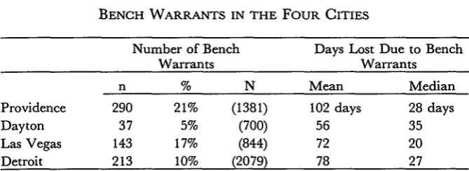
In cases in which a defendant's sanity is under question, the defend-ant is frequently institutionalized in a hospital for a period of observa-tion.26 The period of institutionalization is not time under the control of the court. In the four courts, psychiatric cases take at least twice as long to reach disposition as other cases (see Table 3). For these reasons, psy-chiatric cases were dropped from the analysis of trial court time because that is the phase in which hospitalization and psychiatric exams occur.27 Defendants frequently fail to appear at scheduled court appear-ances. Looking at Table 4, we find that the proportion of cases involv-ing at least one bench warrant ranges from five percent in Dayton to twenty-one percent in Providence. The time during which a defendant is not available is outside the court's control.28 Thus, it is appropriate to adjust the case processing time variable to subtract time lost due to war-rants at whichever stage such loss of time occurred. The subtraction procedure is used rather than excluding these cases because the number of such cases is not trivial and because the time lost due to the failure to appear can be accurately determined. The time loss resulting from the issuance of a warrant can be quite substantial. In Providence, the me-dian number of days lost due to warrants was twenty-eight days; the mean, however, was 102, indicating that a few defendants were missing for very long periods.29 In Providence, subtracting this time has a sub-stantial effect. Estimates decrease by one full month-the median of 133
days drops to 101 for total case processing time. In the other cities, how-ever, estimates were reduced by seven days or less.30
26 This period (often mandated by statute) may consume thirty, sixty, or even ninety
days.
27 By contrast, psychiatric cases proceed as quickly as other cases in the lower courts.
Thus, these cases are retained in the analysis of lower court time.
28 It cannot be argued that the court is to blame for defendants skipping in the first place.
Numerous studies have concluded that the type of pre-trial release-own recognizance versus bond-is unrelated to failure-to-appear rates. See, e.g., P. WICE, FREEDOM FOR SALE (1974).
29 If defendants were never apprehended, the cases have been excluded because they lack
a final disposition date. In many other cases, defendants reappear subsequent to the issuance of a bench warrant. A simple summary measure can be misleading. While defendants in a significant proportion of warrant cases are missing for only brief periods, some were missing for periods of two years or more.
30 Excluding psychiatric cases from the analysis and subtracting days lost due to warrants
DAVID W NEUBA UER
TABLE 4
BENCH WARRANTS IN THE FOUR CITIES
Number of Bench Days Lost Due to Bench
Warrants Warrants
n % N Mean Median
Providence 290 21% (1381) 102 days 28 days
Dayton 37 5% (700) 56 35
Las Vegas 143 17% (844) 72 20
Detroit 213 10% (2079) 78 27
Once corrective actions have been taken, we achieve a more accu-rate measure of case processing time attributable to the actions of the court.3 1 Thus, the impact of the innovations can be better assessed.
C. VARIATIONS IN CASE PROCESSING TIME
The most striking thing about case processing time is its variability; some cases reach disposition soon after filing while others may languish for years. Understanding variations in case processing time is vital. Past studies have used one or more statistical measures: mean, median, and/or the toughest ten percent.3 2 These efforts have failed to present and analyze important variations in case processing time, since no single statistical measure can capture the full range of variation. One instead must examine case processing time with a variety of statistical measure-ments to detect important variations in case duration.33
In statistics, the most commonly used summary measure is the
31 Some other events, idiosyncratic to a particular site---such as a habeas petition to the
Nevada State Supreme Court-were also deemed to be outside the court's control. This time was likewise subtracted out.
32 T. CHURCH, supra note 11; S. FLANDERS, E. HOLLEMAN, J. LEDERER, J. McDERMOTT
& D. NEUBAUER, CASE MANAGEMENT AND COURT MANAGEMENT IN UNITED STATES DIs-TRICT COURTS (1977); S. WASBY, T. MARVELL & A. AIKMAN, VOLUME AND DELAY IN STATE APPELLATE COURTS: PROBLEMS AND RESPONSES (1979) [hereinafter cited as S. WASBY].
33 This approach reflects currently popular analysis and display techniques from
"explor-atory data analysis" (EDA) developed in J. TUKEY, EXPLORATORY DATA ANALYSIS (1977);
see also P. HARTWIG & B. DEARING, EXPLORATORY DATA ANALYSIS 9 (1979):
The underlying assumption of the exploratory approach is that the more one knows about the data, the more effectively data can be used to develop, test, and refine theory. Thus, the explanatory approach to data analysis seeks to maximize what is learned from the data, and this requires adherence to two principles: skepticism and openness. One should be skeptical of measures which summarize data since they can sometimes conceal or even misrepresent what may be the most informative aspects of the data, and one should be open to anticipated patterns in the data since they can be the most revealing outcomes of the analysis.
[image:11.454.67.402.59.181.2]mean (arithmetic average). Means are sometimes used to measure case processing time, but they do not provide a good portrayal of a "typical" case since they are heavily influenced by a handful of extreme values. Particularly in court delay studies, the mean gives undue weight to a few cases that take a relatively long time to reach disposition.
Because the mean can hide important variations, it is common to report the standard deviation (s.d.) in addition to the mean. The stan-dard deviation is a measure of dispersion of the data around the mean. The extremely high standard deviations in Table 5 are quite obvious. Standard deviations that approach the level of the mean itself are a warning that interpretation of the mean may be problematic.
TABLE 5
TRIAL COURT CASE PROCESSING TIME PRIOR TO
DELAY-REDUCTION PROGRAMS
Standard Baseline Period Mean Median Deviation N Providence Jan.-Dec., 1976 365 days 277 days 345 362
Dayton July-Oct., 1978 82 69 60 265
Las Vegas Jan.-March, 1977 102 61 138 74
Detroit April-Oct., 1976 105 55 111 440
The median is a better summary measure of case processing time,34 and for that reason it has been used exclusively in the past. A median indicates that half of the cases took more time and half took less than the median score. Because the median is less influenced by a handful of extreme cases, it typically provides a lower estimate of case processing time than the mean. Table 5 provides data for each city's trial court time in the pre-innovation period only. The Table shows that the me-dian is consistently lower than the mean. Note that for Providence, the difference is substantial (almost ninety days), and in Detroit and Las Vegas the mean is nearly twice as long as the median trial court time. Only in Dayton is the difference between the mean and the median rela-tively small (thirteen days). Thus, the view of case processing time dif-fers considerably depending upon which statistical measure-the mean or the median-is employed.
[Vol. 74
0
0
0
F-z
U,
p
0 U
C) C C> C, (1
C)O
1600 DAVID W. NEUBA UER
*0 ' *
0 10
- 0
Box-and-whisker plots, developed by Tukey,3 5 are another effective method of displaying information about the entire range of a variable.3 6 Whereas means and medians attempt to summarize the central ten-dency of a variable, a box-and-whisker plot provides information about cases surrounding the median and extreme cases as well. Figure 1 presents box-and-whisker plots for the pre-innovation period in our four sites.
The "box" represents the range of the cases falling between the twenty-fifth percentile and the seventy-fifth percentile. The size (length) of the box is a visual summary of the range in values: the larger the box, the greater the range; the smaller the box, the more constricted the range. The horizontal line inside the box is the median value-the age of the case(s) at the fiftieth percentile.
The boxes highlight interesting differences in case processing time between the four sites. In Providence, not only do cases take longer on an average to reach disposition, but the range is also great. This sug-gests that the process is less routinized than in the other three cities. A less drastic, but nonetheless important, difference between Las Vegas and Dayton also becomes apparent. Comparison of the medians indi-cates that the cities are about the same (median of sixty-nine for Dayton and sixty-one for Las Vegas). However, the range in Las Vegas is much greater. Fully twenty-five percent of the cases are disposed of quickly (eight days), but cases at the seventy-fifth percentile take longer than in Dayton. In short, the Las Vegas distribution is skewed at both ends. Scrutiny of the bottom hinge (twenty-fifth percentile) reveals another important dimension of case processing time: all four courts were able to dispose of a fair proportion of cases relatively quickly. Even in Provi-dence, one quarter were disposed of within one and one-half months. Note that in Las Vegas and Detroit, the courts produced a fairly large proportion of very early guilty pleas.
The "whisker" represents the value of an outlier, an extreme case. Some distributions may have numerous outliers, at the upper end (above the box) or at the lower end (below the box). The whiskers con-note outlying values to facilitate substantive interpretation. Therefore, we have included only one whisker atop the line extending down to the box. This whisker, in our analysis, represents the value of the case(s) lying at the ninetieth percentile. This allows us to determine how long the courts' long cases take to process.
35 J. TUKEY, supra note 33.
DAVID W NEUBA UER [Vol. 74
-.
G~C- - - C C
The contrast between the four sites is again instructive. In Las Vegas, the ninetieth percentile case took 228 days, which was less than the median case processing time in Providence. Dayton and Las Vegas differ far more than either the mean or median would suggest. Cases at the ninetieth percentile are disposed of two months earlier in Dayton than in Las Vegas. Detroit was marked by a higher-than-expected pro-portion of long cases. While the median time in Detroit was the fastest, it had more long cases than either Dayton or Las Vegas. The central advantage of the box-and-whisker technique is that it provides a good visual summary of important variations in case processing time.
D. CHANGES OVER TIME
Often, one is interested not only in the duration of cases, but also in changes over time. The most fundamental question is whether case processing time decreases after the introduction of delay reduction programs.
A basic way of examining time-series data is through a time line-a graph indicating the value of the observed variable over several points in time. Since this Research Note is not concerned with substantive in-terpretations but rather with conceptual and methodological problems, it is easiest to depict changes over time by using data from just one court. Figure 2, therefore, provides a time line for Providence, using both mean and median values.37 Providence was chosen because that
court underwent the greatest degree of change and therefore provides the most illustrative material.
Median values are likely to fluctuate less than mean values. Never-theless, there may be substantial fluctuation from month to month be-cause the sample size is typically small.38 Ascertaining a trend in such data may not be easy, at least not by mere visual inspection. Tukey pioneered a method of "smoothing" data to provide a "clearer view of the general, once it is unencumbered by details."'39 One way to smooth
37 The time lines displayed in Figures 2 and 3 differ in an important way from most time-series data. Time-time-series analysis is typically based on a quasi-experimental design. After a certain period, a new program is put into effect. The data points prior to the innovation serve as a baseline, while those after seek to measure the impact, if any, of the program. These data points would either follow a group through the program or would be based on non-reactive measures (numbers of highway accidents, for example). Our time-series, however, does not display these independent measures, for the innovations also worked on cases filed (but not disposed of prior to the innovation. Thus, our base period is contaminated. As a result, the base periods often look better than they would have if the innovations had not been insti-tuted. In addition, downturns in trend lines may start before the innovations are put into place. This may suggest anticipatory impact, but may also reflect a statistical artifact.
38 Detroit is the exception; approximately 80 cases per month comprise the sample in this site.
1604 .DAVID W4. NEUBA UER [Vol. 74
"0I"
:
0
-. 0
0
z
-,-.-- '1=
zz
-,-c'_,"
A.:
[.=, , 0
C-ac
fluctuating values over time is through the use of "running medians," a technique which takes a median of surrounding medians, thereby cast-ing to one side extreme median values.4 Figure 3 illustrates a time line
FIGURE 4
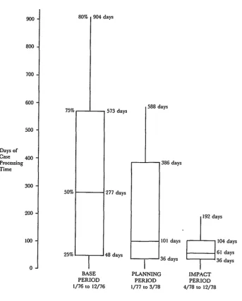
BOX-AND-WHISKER PLOT OF CASE PROCESSING TIME IN PROVIDENCE, BY TIME PERIOD
900 80% 904 days
800
700
600 588 days
75% 573 days
500
Days of Case 400
Processing 386 days
Time
300
50% 277 days
200 192 days
100 101 days 104 days
25% 48 days 61 days
6
"days 36 days
BASE PLANNING IMPACT
PERIOD PERIOD PERIOD
1/76 to 12/76 1/77 to 3/78 4/78 to 12/78
40 The actual computation of the running median is quite simple. The specific technique,
[image:18.454.51.395.140.568.2]DAVID W NEUBA UER
connecting running medians for the median values indicated in Figure 2. The result is a vastly clearer picture of the general-a significant downward sloping trend in case processing time. Through this method, one can still get a picture of the "rough" or residuals by examining the distance between the actual median (marked by an "." in Figure 3) and the running median for any time point.
While the running median provides a useful overview, we also need to examine dispersion. A box-and-whisker plot for every month's sam-ple of cases would be impractical, both logistically and visually. We have therefore divided time spans into either two or three periods, which roughly correspond to key transitions in our courts. Thus, the first time period is always the baseline period, and later time periods may reflect planning and impact periods (as in Providence).
By comparing the box-and-whisker plots in several different time periods, we can identify a number of changes. We can see changes in a court's handling of tougher cases by examining shifts in the top of the box (seventy-fifth percentile) and the location of the whisker (ninetieth percentile). Finally, we are able to inspect changes in the size of the boxes across time periods. We would expect that in courts which im-prove their processing of cases, the size of the boxes would become smaller. Cases would be processed more uniformly in time, especially in the middle fifty percent of a court's cases. The upper tails (whiskers) also should drop sharply, as the amount of time needed to process the longest ten percent of a court's cases decreases.
Figure 4 illustrates these expectations for Providence. The earlier use of the running median indicated that, overall, case processing time declined after the introduction of the delay reduction programs. We now see that the effects extended far beyond a decrease in the median. The strikingly smaller size of the box indicates that delay reduction was felt across the entire range of cases. Case processing time became more uniform. Moreover, the number of cases taking a very long time to reach disposition declined dramatically. The ninetieth percentile now stands at 192 days, a decrease of over one and one-half years from the baseline period.
III. CONCLUSION
The determination of case processing time is as elusive as it is im-portant. As research on court delay emerges from infancy, a host of subsidiary research problems arise. What one chooses to measure and which statistical measurements one chooses have important
conse-quences for the determination of case processing time.
Analyzing total case processing time provides too gross a measure because it lumps together separate and distinct phases. It is far prefera-ble to analyze individual time frames: lower court time, trial court time, and sentencing time.
Because not all case processing time is attributable to the court, one needs to measure only "time under the control of the court." We there-fore must exclude cases involving a psychiatric examination because they are few in number and involve significant time not under the con-trol of the court. Similarly, we subtract days lost due to the defendant's failure to appear. These refinements leave us with a set of more "typi-cal" and "routine" cases.