Impact of Microcredit Programs on Female Headed Households in Jimma Zone, Ethiopia

(1)

Impact of Microcredit Programs on Female Headed

Households in Jimma Zone, Ethiopia

Yilkal Wassie Ayen

M.Sc, Lecturer, Jimma University Economics Department

Abstract- Microfinance and microcredit is a recent development issue and one of the mechanisms to empower poor people in rural Ethiopia. Microfinance interventions may empower women by increasing their incomes and their control over that income. This study evaluates the impact of microcredit program on female headed households’ annual expenditure in rural Ethiopian, Jimma Zone. Data were collected from 1092 female headed households from both participants and non-participants in microcredit program during 2013. Data was analyzed using the PSM technique. PSM results show that participant in microcredit program has a significant and positive impact on households’ annual expenditure. Furthermore, the Probit result sows that higher price of egg and sugar makes households more likely to participate in microcredit program. However, more educated households’, large land holders and higher income earners are less likely to participate in the program.

Index Terms- Female Headed Households, Microcredit Participation and Propensity Score Matching

I. INTRODUCTION

any studies often defined the terms microcredit and microfinance interchangeably, however it is important to recognize the distinction between the two. Microcredit defined as the practices of delivering financial loan to poor clients. On the other hand Microfinance is the act of providing these same borrowers with financial services, such as saving and insurance policies. In short, microfinance encompasses the field of microcredit (Sengupta et.al 2008).

Microfinance institutions (MFIs) take in a wide range of providers that vary in legal structure, mission, and methodology to offer these financial services for poor clients who do not have access to mainstream banks or other formal financial service providers (Gutu, 2014). Microfinance is a kind of service that serve as the supply of loans, savings, money transfers, insurance, and other financial services to low-income people. Microfinance is a place for the poor and near poor clients to get access to a high quality financial service, which include not just credit but also savings, insurance and fund transfers.

However, Microcredit or known as micro lending is defined as an extremely small loan given to poor people to help them become self employed (Nawai and Shariff, 2010). Microcredit was given to the underprivileged individuals for income-generating activities that will improve the borrowers’ living standards. The loan characteristics are, too small, short-term credit (a year or less), no collateral required, weekly repayment, poor borrower and mostly women who are not qualified for a

conventional bank loan. Usually the loan pays high interest rates because of the high cost in running microcredit program and high risk associated with it.

Since collateral is often not required, the effectiveness of the program becomes the main issue for the microcredit institutions to continue providing this services. This is because most of the microcredit institutions are Non- Governmental Organizations (NGOs), that received funds from the government and donors and they are not profit oriented organizations (Ibid).

Beginning in the mid-seventies, savings and credit institutions started extending small loans to groups of poor women in the villages in order to empower them to invest in microenterprises. This form of micro-enterprise credit is based on solidarity group lending where every group member is tasked to ensure the repayment of all members (Gutu, 2014). This would have been one solution to reduce risk associated with this service. However, regarding delivery of financial service, access to women’s credit was very limited in Ethiopia. Because of this limited access, the majority of the poor get financial services from informal sources: like money lenders, Iqub1, Iddr2, merchants, friends and relatives etc. The formal financial institutions have not been interested in delivering credit to the poor because of collateral requirements (Abafita. 2003).

Like in other areas of the world, people in Ethiopia are living under poverty. Financial institutions in general, microfinance programs in particular play a crucial role in the empowerment of poor women. However, studies on the impact of microfinance participation by women were extremely limited. Thus, this study has been undertaken to analyze the impact of microfinance participation on female headed households. Furthermore this study tried to understand the institutional and socio-economic factors that affect microfinance program participation in the area and the extent to which this program participation would improve the consumption expenditure of the households.

Problem Statement and Research Question

Benefiting women from microfinance credit schemes is a targeting technique to supplement subsistence level of

1

Iqub is a regular type of social connection in Ethiopia; basically a group of people together collect equal amount of money and distribute that money term by term for each members. Members of the group used the money to run a business or often to smooth their consumption.

2

Iddr is another form of social institution in Ethiopia that basically serves as traditional insurance for those people in the member.

(2)

agricultural production and empower them in rural Ethiopia. Micro-finance interventions may empower women by increasing their incomes and their control over that income, enhancing their knowledge and skills in production and trade, and increasing their participation in household decision-making like on expenditure. As a result, social attitudes and perceptions may change, and women’s status in the household and community may be enhanced (Kabeer, 1996).

The active participation of women in agriculture is the recent phenomena of rural economic development. Nweze (1995) observed that rural women: are too poor to save, lack ability to organize financial self-help activities and need cheap credit to expand production and income in their farms and non-farm activities. Nwajiuba (1999) put emphasis on the centrality of credit, especially for women farmers to increase their investment in the absence of adequate savings. Credit is a critical input because it can be used to overcome financial obstacles. However, women farmers were perpetually marginalized in the institutionalized credit programmers in Ethiopia.

Many development programs have been extending reasonable amount of credits to rural women since. However, factors contributing to the low economic performance of rural women and the effect of microfinance program participation were not yet studied. In this study, the main objective of propensity score matching was microfinance program participation, the treatment (microfinance participation by female headed households) and potential outcome (annual expenditure by households). The idea was to match those women microfinance participants with that of a control group (non participant women) sharing similar observable characteristics. The mean effect of microfinance participation would calculate as the average difference in expenditure between participants and non participants i.e. the impact would the change in household annual expenditure as outcome indicator. The use of PSM method was used to answer the question: what would be the total annual expenditure of female headed households had these households not participated in microcredit services?

Empirical Literature

A majority of microfinance programs generally target women often more financially responsible at repaying than men counter parts. Providing and empowering them should be the main policies of microfinance programs (Setboonsarng et. al, 2008). Even though, women are not explicitly excluded from the credit services in developing countries, they have received practically no credit from the formal financial institutions (Ibid). Several reasons were given by researchers in this regard. First, credit services are administered by socio-cultural reasons and women are passive participants in every village. Second, microfinance service is often at the recommendation of the agricultural extension agents whose contacts are primarily with men. Third, formal financial institutions require collateral for their loan since most type of businesses done by poor people especially women are more risky (Ibid). But the property right of most developing countries favored for men as compared to women. Thus women are by default excluded from such microfinance and microcredit programs. Furthermore, lending institutions usually demand a financial guarantee for any loan, of which women are rarely capable.

Most empirical researches on microfinance have been done to assess the repayment performance of borrowers and were considered more or less the same socio-economic characteristics. Berhanu (2005) while studying on the factors that affect loan repayment performances, by employing the Tobit model, variables like land holding size of the family, agro-ecology of the area, total livestock holding, number of years of experience, number of contacts, sources of credit and income from off-farm activities are found to be significant in affecting loan repayment performance. However, the other variables (family size, distance between main road and household residence, purpose of borrowing, loan amount and expenditure for social festivals) are found to be insignificant variables.

Women borrowers in rural areas of Ethiopia used microfinance services for consumption smoothing purposes and they encountered default. They used this income for financing social ceremonies and would not empower them. Assefa (2002) employed a logit model to estimate the effects of hypothesized explanatory variables on the repayment performance of rural women credit beneficiaries in Dire Dawa, Ethiopia. Variables like farm size, annual farm revenue, celebration of social ceremonies, loan diversion, group effect and location of borrowers from lending institution are found to be statistically significant in affecting the loan repayment performance. Retta (2000, cited in Abafita, 2003) employed probit model for loan repayment performance of women fuel wood carriers in Addis Ababa. His finding is that of loan, supervision, suitability of repayment period and other income sources are found to encourage repayment hence reduce the probability of loan default. While educational level is negatively related to loan repayment.

Belay (2002), used a binary Logit model to analyze factors influencing loan repayment performance of rural women. Location of borrowers from lending institution, loan diversion, annual farm revenue and celebration of social ceremonies were highly important in affecting loan repayment performance. In addition Reta (2011) found that age and business types were important in influencing loan repayment performance of the borrower. In addition, gender and business experience of the respondents were found to be significant determinants of loan repayment rate.

Ughomeh et.al (2008) investigated the determinants of loan repayment performance among women self-help groups in Bayelsa State, Nigeria. The study revealed that credit was available for agricultural production, processing and petty trading among women farmers. Loan repayment percentage was determined to be 83.73% while percentage default was 17.27%. The estimated regression model indicated that women as household heads, interest rate and household size, negatively and significantly affected the loan repayment performance while price stability of farm proceeds and commitment to self help groups, positively and significantly affect the loan repayment of women farmers in self help groups in the area.

(3)

income generation activities such as agricultural production and, in particular, animal raising. However, the impacts on education, health, female empowerment, and so forth were of limited significance.

In addition some other empirical researches confirmed that microfinance participation improve the welfare of participant households. Ghalib et, al (2011), in their study in Pakistan employ a quasi-experimental research design and make use of the data collected by interviewing both borrowers and non-borrower households and control for sample selection biases by using propensity score matching. In this study household access to microfinance reduce poverty. It has been confirmed that microfinance programs had a positive impact on the welfare of participating households.

Arun et,al, (2006), applied propensity score matching method in their to analyze the effect of Micro Finance Institutions (MFIs) on poverty reduction of households in India. The propensity score matching method was employed to estimate the poverty reducing effects of the access to microfinance institutions. Significantly positive effects on the multidimensional poverty indicator suggest the role of microfinance institutions in poverty reduction. It also showed that households in rural areas need loans from microfinance for productive purposes to reduce poverty, while simply accessing to microfinance program is sufficient for urban households to reduce it.

In general, most empirical researches on female headed households have been done on loan the repayment performance. However, few other research outcomes also studied on the

impact of microcredit program participation on rural people though researchers used different variables in their empirical findings. Hence, empirical studies on female headed households are scanty. Therefore, this study has been conducted to contribute in the economic literature on the impact of microcredit program participation on female headed household annual expenditure in Ethiopia.

II. METHODOLOGY

This part presents the research methodology. It describes the data collected and the specific procedures used in evaluating the impact of microcredit program participation on female headed households by using PSM.

Data and Data Collection Procedure

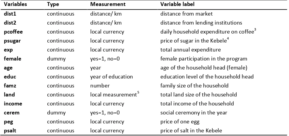
[image:3.612.66.548.426.653.2]

The data used in this study was collected from three microfinance (Eshet, Harbu and Oromia) around Jimma zone, Ethiopia. The data was collected by loan officers of each micro-finance for a special use during 2014. Information was collected from sample women microfinance participants and non-participants during 2013 about their socio-economic characteristics like family resource level (income), distance from market, distance from lending institutions, price of marketable products, etc, and individual characteristics; age, education status and family size was obtain through questionnaires.

Table 1: Description of variables and measurement

Variables Type Measurement Variable label

dist1 continuous distance/ km distance from market

dist2 continuous distance/ km distance from lending institutions pcoffee continuous local currency daily household expenditure on coffee3 psugar continuous local currency price of sugar in the Kebele4

exp continuous local currency total annual expenditure

female dummy yes=1, no=0 female participation in the program

age continuous year age of the household head (female)

educ continuous year of education education level of the household head

famz continuous number family size of the household

land continuous local measurement5 total land size of the household income continuous local currency total income of the household

cerem dummy yes=1, no=0 social ceremony in the year

peg continuous local currency price of one egg

psalt continuous local currency price of salt in the Kebele

Source: own computation

3

Every day average estimated coffee consumption expenditure of households measured in Ethiopian birr. 4

(4)

Empirical Model

In most studies propensity score matching method has been used to evaluate public policies and programs. This method enable researchers to extract information from the sample of microfinance participants (treated) households and a set of matching households that look like the non participant (controlled) households in all relevant pre-intervention characteristics. In other words, PSM matches each adopter household with a non-participant household that has almost the same likelihood of adopting any social programs. The aim of matching is to find the closest comparison group from a sample of nonparticipants to the sample of microfinance service participants.

In this study program participation (Microcredit

participation) indicator equals one if individual i participated and zero otherwise. The treatment effect for an individual i written as:

6

[1]

The fundamental evaluation problem arises because only one of the potential outcomes is observed for each individual i. The unobserved outcome is called counterfactual outcome.

The average treatment effect (ATT) is that the parameter that received the most attention in evaluation literature, which is defined as:

[2]

As the counterfactual mean for those being treated

is not observed, one has to choose a proper substitute for it in order to estimate ATT. Using the mean

outcome of untreated individuals is in non-experimental studies usually not a good idea, because it is most likely that components which determine the treatment decision also determine the outcome variable of interest. Thus, the outcomes of individuals from treatment and comparison group would differ even in the absence of treatment leading to a `self-selection bias'. For ATT it can be noted as:

[3]

The difference between the left hand side of equation [3]

and is the so-called `self-selection bias'. The true parameter

is identified:

[4]

6_{The treatment effect for an individual i}

Thus, in a program evaluation literature the effectiveness of matching estimators as a feasible estimator depends on two fundamental assumptions:

Conditional Independence Assumption [CIA]: This assumption imposes a restriction that choosing to participate in a program is purely random for similar individuals. Given a set of observable covariates (X) which are not affected by treatment, potential outcomes are independent of treatment assignment. This assumption implies that the selection is solely based on observable characteristics, and variables that influence treatment assignment and potential outcomes are simultaneously observed.

[5]

It should also be clear that conditioning on all relevant covariates is limited in case of a high dimensional vector X. The

propensity score i.e. the probability for an individual to participate in a treatment given his observed covariates X, is one possible balancing score. The conditional independence assumption (CIA) based on the propensity score (PS) can be written as:

[6]

Common Support: A further assumptions besides conditional independence (CIA) is the common support or overlap condition. The assumption is that P(x) (probabilities) lies between 0 and 1. This restriction implies that the test of the balancing property is performed only on the observations whose propensity score belongs to the common support region of the propensity score of treated and control groups (Becker and Ichino, 2002). Individuals that fall outside the common support region would be excluded in the treatment effect estimation. This is an important condition to guarantee improving the quality of the matching used to estimate the ATT.

(Overlap) [7]

Common support ensures that individuals with the same characteristics have positive probability of being treated or not treated in the program.

Finally the PSM estimator for ATT can be written as:

[8]

(5)

Choosing Matching Algorithm

All matching estimators contrast the outcome of a treated individual with outcomes of controlled group members. PSM estimators differ not only in the way the neighborhood for each treated individual is defined and the common support problem is handled, but also with respect to the weights assigned to these neighbors.

Nearest Neighbor Matching: The most straightforward matching estimator is nearest neighbor (NN) matching. The individual from the comparison group is chosen as a matching partner for a treated individual that is closest in terms of propensity score. A problem which is related to NN matching without replacement is that estimates depend on the order in which observations get matched. Hence, when using this approach it should be ensured that ordering is randomly done. Caliper and Radius Matching: NN matching faces the risk of bad matches, if the closest neighbor is far away. This can be avoided by imposing a tolerance level on the maximum propensity score distance (caliper). To overcome this problem the caliper matching algorithm is another alternative. Caliper matching means that an individual from the comparison group is chosen as a matching partner for a treated individual that lies within a given caliper (propensity score range) and is closest in terms of propensity score (Caliendo and Kopeinig, 2008). Imposing a caliper works in the same direction as allowing for replacement. Bad matches are avoided and hence the matching quality rises. However, if fewer matches can be performed, the variance of the estimates increases.

Stratification and Interval Matching: The idea of stratification matching is to partition the common support of the propensity score into a set of intervals (strata) and to calculate the impact within each interval by taking the mean difference in outcomes between treated and control observations. Clearly, one question to be answered is how many strata should be used in empirical analysis.

Kernel and Local Linear Matching: The matching algorithms discussed so far have in common that only a few observations from the comparison group are used to construct the counterfactual outcome of a treated individual. Kernel matching (KM) and local linear matching (LLM) are non-parametric matching estimators that use weighted averages of all individuals in the control group to construct the counterfactual outcome. Thus, one major advantage of these approaches is the lower variance which is achieved because more information is used. A drawback of these methods is that possibly observations are used that are bad matches. Hence, the proper imposition of the common support condition is of major importance for KM and LLM.

Assessing the Matching Quality

Since we do not condition on all covariates but on the propensity score, it has to be checked if the matching procedure is able to balance the distribution of the relevant variables in both the control and treatment group. Several procedures to do so are discussed in this subsection. These procedures can also, as already mentioned, help in determining which interactions and higher order terms to include in the propensity score specification for a given set of covariates. The basic idea of all approaches is to compare the situation before and after matching

and check if there remain any differences after conditioning on the propensity score. If there are differences, matching on the score is not (completely) successful and remedial measures have to be done, e.g. by including interaction-terms in the estimation of the propensity score. The followings are common criteria to assess the matching qualities.

Standardized Bias: One suitable indicator to assess the distance in marginal distributions of the variables is the standardized bias (SB). For each covariate X it is defined as the difference of sample means in the treated and matched control subsamples as a percentage of the square root of the average of sample variances in both groups. The standardized bias before matching is given by:

[9]

The standardized bias after matching is given by:

[10]

Where X1 (V1) is the mean (variance) in the treatment group before matching and X0(V0) the analogue for the control group. X1M (V1M) and X0M (V0M) are the corresponding values for the

matched samples.

t-test: A similar approach uses a two-sample t-test to check if there are significant differences in covariate means for both groups (Rosenbaum and Rubin, 1985). Before matching differences are expected, but after matching the covariates should be balanced in both groups and hence no significant differences should be found. The t-test might be preferred if the evaluator is concerned with the statistical significance of the results. The shortcoming here is that the bias reduction before and after matching is not clearly visible.

Joint Significance and Pseudo-R2: Additionally, Sianesi (2004) suggests re-estimating the propensity score on the matched sample that is only on participants and matched non-participants and compare the pseudo-R2's before and after matching. The pseudo-R2 indicates how well the repressors X explain the participation probability. After matching there should be no systematic differences in the distribution of covariates between both groups and therefore, the pseudo-R2 should be fairly low.

Therefore, this study follows and adopts the appropriate empirical methodology. The necessary estimation techniques along with PSM method were used. It describes the average treatment effect; the common support regions; the matching algorithms and the matching quality are presented.

III. RESULTS

(6)

(VIF) was calculated to check the problem of multicollinearity among explanatory variables (see appendix A), all explanatory variables are significantly far below 10 (no serious problem of multicollinearity). STATA 13 version software was used to estimate the PSM model and the effect of microfinance program participation on the annual expenditure of female headed households. The PSM model tried to match 520 controlled female headed households with 572 treated one.

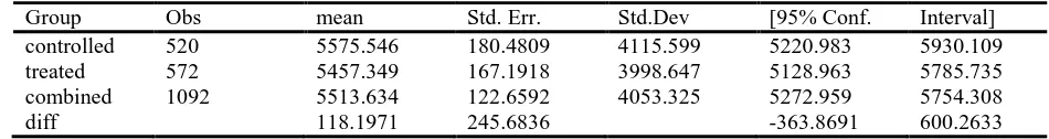
Table2: Simple Comparison of Treated and Controlled Households by Expenditure

Group Obs mean Std. Err. Std.Dev [95% Conf. Interval]

controlled 520 5575.546 180.4809 4115.599 5220.983 5930.109

treated 572 5457.349 167.1918 3998.647 5128.963 5785.735

combined 1092 5513.634 122.6592 4053.325 5272.959 5754.308

diff 118.1971 245.6836 -363.8691 600.2633

Source: Own computation

There is no mean significance difference between the treated and controlled households. From the above table we observed that the comparison and controlled households almost had the balanced number of observations and it makes the analysis more robust.

Estimation of Propensity Scores

The first stage in the propensity score matching is to estimate the probability of being a microcredit or microfinance participant. For this purpose, this study considered variables that influence the likelihood of borrowing from microfinance. The rationale behind this is that, if a variable influences participation but not the outcome, there is no need to control for differences with respect to this variable in the treatment versus the control groups. Likewise, if the variable influences the outcome but not the treatment likelihood, there is no need to control for that variable since the outcome will not significantly differ in the treatment versus the control groups. Variables that affect neither treatment nor the outcome are also clearly unimportant

(Setboonsarng et. al, 2008). Therefore, only those variables that influence both the treatment and the outcome are needed for the matching and are included in the Probit model.

[image:6.612.66.541.172.235.2]

Thus, the Probit regression model was used to estimate the propensity score matching for participant and non-participant female headed households. The dependent variable is binary that indicate households’ participation in microfinance and microcredit services. Results presented in Table 3 below shows the estimated model appears to perform well for the intended matching exercise because the pseudo-R2 value is 0.0608. A low R2 value shows that program households do not have much distinct characteristics overall (Tolemariam, 2010) and as such finding a good match between program and non-program households becomes easier.

Table 3: Probit Regression Result

female Coef. Std. Err. Z P>[Z] [95% Conf. Interval]

dist1 .0009575 .0157137 0.06 0.951 -.0298408 .0317558

dist2 -.024542 .0375957 -0.65 0.514 -.0982282 .0491442

pcoffee .1735661 .1355659 1.28 0.200 -.0921383 .4392704

psugar .0212326 .0101011 2.10 0.036** .0014348 .0410304

age .0039881 .003261 1.22 0.221 -.0024034 .0103796

educ -.0405907 .0124198 -3.27 0.001*** -.0649332 -.0162483

famz -.0017576 .0190778 -0.09 0.927 -.0391494 .0356341

land -.001512 .0004622 -3.27 0.001*** -.0024178 -.0006061

income -4.66e-07 2.35e-07 -1.98 0.048** -9.28e-07 -4.43e-09

cerem -.2026552 .1088702 -1.86 0.063* -.416037 .0107266

peg .3309907 .1347578 2.46 0.014** .0668702 .5951112

psalt .034816 .0490617 0.71 0.478 -.0613432 .1309752

(7)

Number of obs 1092

LR chi2 (12) 91.82

Prob > chi2 0.0000

Pseudo R2 0.0608

***, ** and * is significant at %1, 5% and 10% level of significance respectively

Source: Own computation

Looking into the estimated coefficients above, the results indicate that program participation is influenced by six explanatory variables. Price of sugar, education level of the household, land size, annual income, social ceremony per year and price of egg variables are which affect the participation of the household to the microfinance program. In this probit regression result some variables like price of egg and price of sugar are makes households more likely to participate in microfinance program. On the contrary, more educated households’, those households with large land size and higher

income households are less likely to participate in the program. In addition, social ceremony celebrators are less likely to participate in the program (at 10% level of significance).

Common Support

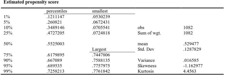
[image:7.612.70.545.365.524.2]

The final number of blocks in this model is 4. This number of blocks insures that the mean propensity score is not different from treated and controls in each blocks. The region of common support is [0.05302391, 0.77618416] implying that the two groups share the same characteristics in these brackets.

Table 4: Region of Common Support

Estimated propensity score

percentiles smallest

1% .1211147 .0530239

5% .260821 .0672431

10% .3489146 .0705541 obs 1082

25% .4727205 .0724818 Sum of wgt. 1082

50% .5525003 mean .529477

Largest Std. Dev .1287829

75% .6179895 .7447806

90% .667089 .7588135 Variance .016585

95% .689535 .7757975 Skewness -1.162977

99% .7258213 .7761842 Kurtosis 4.4563

Source: Own computation

Matching Algorithm

Alternative matching estimators were used in matching the treatment and control households in the common support region. The following result (Table 5) shows that female microfinance participation does have a significant impact on household per capita expenditure by the nearest-neighborhood matching method at 5 percent level of significance (t = 2.242). The average treatment effect of the treated (ATT) on household expenditure for female headed program participation was 611.699. Participants are on average more annually expend Birr 611.699 as compared to non participants.

The average treatment effect using stratification matching result that follows shows 555.598 more annual expenditure of female head household because of program participation. The impact is significant at 5 percent level (t = 2.646). Furthermore, the ATT using radius matching result shows an increased impact (721.797) more household expenditure significantly (t = 3.097) of women’s microcredit participation on per capita expenditure. The number of individuals matched more or less consistent in all matching algorithms. Looking in to the average treatment effect using kernel matching result is consistent with earlier findings. The robustness of the result of this matching algorithm, women’s participation increases per capita expenditure by 652.645 at a 5 percent significance level. This result was quite similar with nearest neighbor, radius and stratification matching methods.

(8)

Matching type7 n. treat.8 n. contr.9 ATT10 Std. Err. t

NN 572 275 611.699 272.874 2.242**

Stratification 572 510 555.598 210.014 2.646**

Radius 501 399 721.797 233.072 3.097**

Kernel11 572 510 652.645 229.275 2.847**

** Significant at 5% level

Thus, all matching algorithms used above gives similar results. The maximum amount of treated households considered in estimation of ATT was 572 whereas the minimum was 501. The minimum amount of controlled among these matching algorithms was 275 and the maximum 510. The maximum average expenditure because of credit program participation in these matching algorithms was 721.797 while the minimum was 555.598. All results were statistically significant at five percent.

[image:8.612.73.541.246.660.2]

Matching Quality

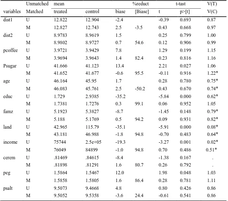
Table 6: Matching Quality

Unmatched mean %reduct t-tast V(T)

variables Matched treated control biase [Biase] t p>[t] V(C)

dist1 U 12.822 12.904 -2.4 -0.39 0.693 0.87

M 12.827 12.743 2.5 -3.5 0.43 0.668 0.97

dist2 U 8.9783 8.9619 1.5 0.25 0.799 1.00

M 8.9802 8.9727 0.7 54.6 0.12 0.906 0.99

pcoffee U 3.9721 3.9429 7.8 1.29 0.199 1.15

M 3.9694 3.9643 1.4 82.4 0.23 0.816 1.16

Psugar U 41.666 41.123 13.4 2.21 0.027 1.06

M 41.652 41.677 -0.6 95.5 -0.11 0.916 1.22*

age U 46.164 45.95 1.7 0.28 0.780 0.75*

M 46.083 45.761 2.5 -50.2 0.43 0.670 0.74*

educ U 1.729 2.9385 -35.2 -5.84 0.000 0.62*

M 1.7381 1.7276 0.3 99.1 0.06 0.952 1.05

famz U 5.1923 5.3827 -8.7 -1.45 0.148 0.79*

M 5.188 5.1769 0.5 94.2 0.09 0.931 0.82*

land U 42.965 115.79 -35.1 -5.91 0.000 0.08*

M 43.181 46.988 -1.8 94.8 -0.70 0.483 0.64*

income U 75744 2.5e+05 -19.3 -3.27 0.001 0.02*

M 76049 84899 -1.0 94.8 0.70 0.486 0.51*

cerem U .81469 .84615 -8.4 -1.38 0.167 .

M .81898 .81291 1.6 80.7 0.26 0.792 .

peg U 1.5864 1.5467 12.0 1.98 0.048 1.03

M 1.5858 1.5805 1.6 86.4 0.28 0.781 1.11

psalt U 9.5073 9.4668 4.8 0.80 0.426 0.86

M 9.5052 9.5358 -3.6 24.4 -0.61 0.541 0.86

7

All matching algorisms; nearest neighbor (NN), Stratification, Radius and Kernel matching are used. 8_{means number of treated observations}

9

number of controlled households

10

Average treatment on the treated

(9)

After choosing the best performing matching algorithm the next task is to check the balancing of propensity and covariates. The main purpose of the propensity score estimation is not to obtain a precise prediction of selection into treatment, but rather to balance the distributions of relevant variables in both groups. The balancing powers of the estimations are ascertained by considering different test methods such as the reduction in the mean standardized bias between the matched and unmatched households, equality of means using t-test and chi-square test for joint significance for the variables used.

The mean standardized bias before and after matching are shown in Table 6 with the total bias reduction obtained by the matching procedure. In all cases, it is evident that sample differences in the unmatched data significantly exceed those in the samples of matched cases. The process of matching thus creates a high degree of covariate balance between the treatment and control samples that are ready to use in the estimation procedure. Similarly, t-values in the same table show that before matching five of chosen variables exhibited statistically significant differences while after matching all of the covariates are balanced.

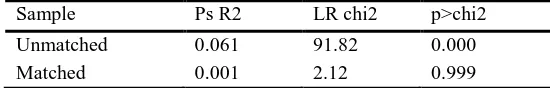
[image:9.612.28.303.472.516.2]

The low pseudo-R2 and the insignificant likelihood ratio tests support the hypothesis that both groups have the same distribution in covariates X after matching (see Table 7). This result clearly shows that the matching procedure is able to balance the characteristics in the treated and the matched comparison groups. We, therefore, used these results to evaluate the effect of microcredit participation of households having similar observed characteristics. This allowed us to compare observed outcomes for participants with those of a comparison groups sharing a common support.

Table 7: Matching Quality with Pseudo R2

Sample Ps R2 LR chi2 p>chi2

Unmatched 0.061 91.82 0.000

Matched 0.001 2.12 0.999

IV. CONCLUSION

In this study data from 1092 female headed households from Jimma zone during 2013 were analyzed by STATA 13 version software. Hence, the study has applied a propensity score matching technique which has become the most widely applied non-experimental tool for impact evaluation of social programs and policies. The main research question of the study was what would have happened to an outcome of interest had the microcredit program not been in place. Answering this question requires observing outcomes with-and-without the program for the same household. However, it is impossible to observe the same object in two states simultaneously.

The result of this study confirms that microcredit participation was significantly affected by six variables; Price of sugar, education level of the household, land size of the household, annual income, social ceremony per year and price of

egg are variables that affect the program participation. Price of sugar and price of egg makes households more likely to participate in the microfinance program. However, more educated households’, those households with large land size and higher income households are less likely to participate in the microfinance program. This is the reason why in rural part of Ethiopia illiterates are more poor than literates and hence thy required more income from credit institutions. Large land size is another source of income in the study area. Therefore, households with large land holdings and higher income earners are less demander of microcredit services.

The propensity score matching based on different matching algorithms have resulted in different number of participant households to be matched with non-participant households after discarding households whose values were out of common support region. The concluding results based on PSM then indicate that there are significant differences in annual expenditure of households between treatment and comparison households, which could be attributed to the participation of microfinance program. Thus microfinance program has positive and significant effect on female headed households’ annual expenditure.

REFERENCES

[1] Abafita, J. (2003). Microfinance and loan repayment performance: A case study of the oromia credit and savings share company (OCSSCO) in Kuyu. Addis Ababa University MSc thesis, Ethiopia.

[2] Arun, T et al. (2006). Does the microfinance reduce poverty in India? Propensity score matching based on nationnal-level household data. Development Economics and public policy working paper series.

[3] Assefa B.A. (2002) ‘Factors influencing loan repayment of rural women in Eastern Ethiopia: the case of Dire Dawa Area’, A Thesis presented to the school of graduate studies, Haromaya Univeristy, Ethiopia.

[4] Becker, S. O. and Ichino, A. (2002). Estimation of average treatment effects based on Propensity Scores: The Stata Journal, 2(4): 1-19.

[5] Belay,A. (2002). Factors Influencing Loan Repayment of rural women In Eastern Ethiopia; The case of Dire Dawa area. MSc Thesis, Haromaya University.

[6] Berhanu A. (2005) ‘Determinants of formal source of credit loan repayment performance of smallholder farmers: the case of north western Ethiopia, North Gondar’. M.Sc. Thesis, Haromaya Univeristy, Ethiopia.

[7] Caliendo, and Kopeinig, (2008). Some Practical Guidance for the Implementation of Propensity Score Matching. IZA Discussion Paper No. 1588. DIW Berlin Department of Public Economics. Königin-Luise-Str. 5, 14195. Berlin. Germany.

[8] Ghalib A.K et al. (2011). The impact of microfinance and its role in easing poverty of rural households: Estimating from Pakistan. Discussion paper series.

[9] Gutu E. (2014). Assessing the effectiveness of group lending and its impact on profitability in case Jimma Zone. MSc Thesis Jimma University, Ethiopia

[10] Kabeer, N. (1996). Agency, well-being and Inequality: Reflections on the Gender Dimensions of Poverty. IDS Bulletin. 27(1). Pp. 11-21.

[11] Nawai. N and Mohdshariff, M (2010). Determinants of Repayment performance in microcredit programs: A review Literature. International Journal of Business and Social Science Vol, 1 No 2

[12] Nwajiuba, C.U. (1999) Adaptive Welfarism: A Paradigm of Policy Driven Development. Owerri Jockel Options Business Bureau.

(10)

[14] Reta F. K. (2011). Determinants of loan repayment performance: a case study in the Addis credit and saving Institution, Addis Ababa, Ethiopia. Wageningen University.

[15] Rosenbaum, P. R. and Rubin, D. B. (1985). Constructing a control group using multivariate matched sampling methods that incorporate the propensity score. The American Statistician, 39(1): 35-39

[16] Sengupta, R. and Aubuchon, C.P. (2008) ‘The Microfinance Revolution: An Overview’, Federal Reserve Bank of St. Louis Review, January/February 2008, 90(1), pp. 9-30.

[17] Setboonsarng et. al (2008). Microfinance and the Millennium Development Goals in Pakistan: Impact Assessment Using Propensity Score Matching, ADB Institute Discussion Paper No. 104

[18] Sianesi, B. (2004). An evaluation of the active labor market programs in Sweden. The Review of Economics and Statistics, 186(1):133-155. [19] Tolemariam A. (2010), Impact assessment of input and output market

development intervention by IPMS project: The case of Gomma Woreda, Jimma Zone. Ethiopia. Thesis Haromaya University

[20] Ugbomeh, M. M. (2008). Determinants of Loan Repayment Performance Among women Self help Groups in Bayelsa State, Nigeria. Agricultural conspectus Scientificus Vol.73 (2008) No. 3

AUTHORS

First Author – Yilkal Wassie Ayen (M.Sc.), Lecturer, Jimma

University Economics Department

Appendix

Appendix A: Test of Multicollinearity among Explanatory Variable

Variable VIF 1/VIF

land 3.32 0.300988

income 3.16 0.316894

dist1 1.86 0.538146

Pcoffee 1.68 0.593643

peg 1.30 0.767529

famz 1.12 0.88999