An investigation into automated processes for
generating focus maps
BRIAN SANJEEWA RUPASINGHE KALUPAHANA ARACHCHIGE
A thesis submitted in partial fulfilment of the requirements of the University of East London
for the degree of Doctor of Philosophy
Abstract
The use of geographic information for mobile applications such as wayfinding has increased rapidly, enabling users to view information on their current position in relation to the neighbouring environment. This is due to the ubiquity of small devices like mobile phones, coupled with location finding devices utilising global positioning system. However, such applications are still not attractive to users because of the difficulties in viewing and identifying the details of the immediate surroundings that help users to follow directions along a route. This results from a lack of presentation techniques to highlight the salient features (such as landmarks) among other unique features. Another problem is that since such applications do not provide any eye-catching distinction between information about the region of interest along the route and the background information, users are not tempted to focus and engage with wayfinding applications. Although several approaches have previously been attempted to solve these deficiencies by developing focus maps, such applications still need to be improved in order to provide users with a visually appealing presentation of information to assist them in wayfinding. The primary goal of this research is to investigate the processes involved in generating a visual representation that allows key features in an area of interest to stand out from the background in focus maps for wayfinding users. In order to achieve this, the automated processes in four key areas - spatial data structuring, spatial data enrichment, automatic map generalization and spatial data mining - have been thoroughly investigated by testing existing algorithms and tools. Having identified the gaps that need to be filled in these processes, the research has developed new algorithms and tools in each area through thorough testing and validation. Thus, a new triangulation data structure is developed to retrieve the adjacency relationship between polygon features required for data enrichment and automatic map generalization. Further, a new hierarchical clustering algorithm is developed to group polygon features under data enrichment required in the automatic generalization process. In addition, two generalization algorithms for polygon merging are developed for generating a generalized background for focus maps, and finally a decision tree algorithm - C4.5 - is customised for deriving salient features,
including the development of a new framework to validate derived landmark saliency in order to improve the representation of focus maps.
Table of Contents
Abstract... i
Table of Contents ... iii
List of Figures ... ix
List of Tables ... xx
List of Abbreviations ... xxiv
Acknowledgements ... xxvi
Dedication ... ...xxvii
Chapter 1 Introduction ... 1
1.1 Research motivation ... 1
1.2 Background ... 4
1.3 Outline of the thesis ... 9
Chapter 2 Research context ... 11
2.1 Focus maps ... 11
2.2 Map generalization ... 14
2.2.1 Knowledge acquisition for generalization ... 15
2.2.2 Conceptual architecture for generalization ... 16
2.2.3 Models of generalization ... 18
2.2.4 Generalization operators ... 19
2.2.5 Generalization algorithms ... 20
2.2.6 Review of the generalization frameworks ... 22
2.2.7 Relationship of generalization models to wayfinding maps ... 25
2.2.8 Related work on building geometries ... 27
2.3 Data enrichment ... 31
2.3.1 Relations in data enrichment ... 32
2.3.2 Clustering ... 33
2.3.3 Related work on clustering building geometries ... 34
2.3.4 Related work on data mining ... 40
2.4 Triangulation ... 41
2.4.1 Delaunay triangulation ... 42
2.4.2 Constrained Delaunay triangulation ... 44
2.4.3 Conforming Delaunay triangulation ... 46
2.4.4 Polygon triangulation ... 50
2.4.5 Related work on building geometries ... 51
2.5 Knowledge discovery ... 53
2.5.1 Data mining methods ... 54
2.5.2 Salient landmarks ... 56
2.5.3 Related work in deriving landmark saliency ... 57
2.6 Problem scope ... 58
2.7 Research objective ... 61
2.8 Research questions ... 61
2.9 Conclusion ... 62
Chapter 3 Research Methodology ... 63
3.1 Related work for the adaptation of research design ... 63
3.2 Research design ... 66
3.3 Methods adopted ... 67
3.3.1 Constrained triangulation spatial data structure ... 67
3.3.2 Spatial clustering of polygons under data enrichment ... 69
3.3.3 Automatic map generalization with building aggregation ... 72
3.3.4 Emphasis of salient landmarks ... 75
3.4 Conclusion ... 78
Chapter 4 Implementation - I: Spatial Data Structure ... 79
4.1 Testing of an existing constrained Delaunay triangulation algorithm ... 80
4.1.1 Input data structure ... 82
4.1.2 Evaluation of the results of constrained Delaunay triangulation ... 83
4.2 Testing of an existing conforming Delaunay triangulation algorithm ... 85
4.2.1 Input data structure ... 85
4.2.2 Enriching Steiner points ... 86
4.2.3 Evaluation of the results of conforming Delaunay triangulation ... 87
4.3 Testing of a new constrained algorithm on polygon triangulation ... 89
4.3.2 Triangulation algorithm ... 89
4.3.3 Evaluation of the results of constrained algorithm on polygon triangulation ... 92
4.4 Testing of a new constrained algorithm on Delaunay triangulation ... 92
4.4.1 Input data structure ... 94
4.4.2 Triangulation algorithm ... 94
4.4.3 Proximity links derivation between polygons ... 102
4.4.4 Evaluation of the results of the constrained algorithm on Delaunay triangulation 103 4.4.5 Validation of the constrained algorithm on Delaunay triangulation ... 105
4.5 Outcome of the triangulation algorithms used for testing ... 106
4.5.1 Constrained Delaunay triangulation ... 106
4.5.2 Conforming Delaunay triangulation ... 106
4.5.3 New constrained algorithm on polygon triangulation ... 107
4.5.4 New constrained algorithm on Delaunay triangulation ... 107
4.5.5 Comparison of the triangulation algorithms ... 107
4.6 Conclusion ... 110
Chapter 5 Implementation - II: Spatial Data Enrichment Process ... 111
5.1 Hierarchical polygon clustering process ... 111
5.2 Automation of hierarchical clustering process ... 113
5.2.1 Derivation of the Gestalt factors... 114
5.2.2 Clustering algorithm ... 120
5.3 Testing of automatic clustering ... 126
5.3.1 Results of automatic clustering ... 128
5.3.2 Synopsis of the contributing algorithms used ... 132
5.3.3 Evaluation of the clustering results ... 133
5.4 Shape enrichment of clusters ... 150
5.4.1 Testing of algorithms for retrieving buildings at the cluster outline ... 150
5.4.2 Testing of new algorithms for the cluster shape enrichment ... 154
5.4.3 Synopsis of the contributing algorithms used ... 161
5.5 Data enrichment workflow ... 161
5.6 Conclusion ... 163
Chapter 6 Implementation - III: Data Mining Process ... 164
6.1 Data enrichment for the Data Mining process ... 165
6.1.1 Automatic derivation of attribute values ... 165
6.2 Data mining approach ... 180
6.2.1 Data pre-processing ... 180
6.2.2 Testing of the data mining algorithms on a synthetic data set ... 181
6.2.3 Testing of the data mining algorithms on a real data set ... 190
6.2.4 Evaluation of the results of the three data mining algorithms ... 195
6.3 Conclusion ... 198
Chapter 7 Implementation - IV: Automatic Map Generalization Process ... 199
7.1 Symbolization algorithm with squaring or enlargement ... 200
7.2 Building cluster aggregation with orthogonal sides ... 202
7.2.1 Creating amalgam with dilation and erosion ... 202
7.2.2 Creating amalgam with concave hull generation ... 205
7.2.3 Squaring edges of the amalgam ... 205
7.2.4 Testing of amalgams after squaring edges ... 208
7.2.5 Enlargement of narrow sections and juts ... 210
7.2.6 Simplification of granular edges ... 214
7.2.7 Testing of amalgams after complete generalization process ... 217
7.2.8 Modified building aggregation algorithm with orthogonal sides ... 222
7.2.9 Testing of amalgams with the modified algorithm ... 226
7.3 Building cluster aggregation with non-orthogonal sides ... 230
7.3.1 Aggregation algorithm with triangulation ... 230
7.3.2 Simplification algorithm ... 238
7.3.3 Testing of building cluster aggregation with non-orthogonal sides ... 238
7.4 Conclusion ... 244
Chapter 8 Results and discussion ... 245
8.1 Dealing with issues in generating the results for focus maps ... 246
8.1.1 Fixing issues in building clustering ... 246
8.1.2 Fixing issues of enrichment of building information for deriving salient landmarks .... ... 248
8.1.3 Fixing issues in the aggregation algorithms developed ... 251
8.1.4 Fixing issues in the simplification of aggregated amalgams ... 254
8.1.5 Further incorporation and development of generalization tools required for deriving focus maps ... 255
8.2 Results of focus maps ... 255
8.2.1 Specifications used in the focus map generation process ... 265
8.2.2 External validation of the results of generalization ... 267
8.2.3 External validation of the results of landmark saliency ... 277
8.3 Discussion ... 313
8.4 Conclusion ... 326
Chapter 9 Conclusions ... 327
9.1 Findings ... 327
9.2 Contribution ... 331
9.3 Future research ... 334
Bibliography ... 335
Appendices ...350
A Prototypes of Graphical User Interfaces with proprietary software ... 350
A.1 Input file creation for constrained Delaunay triangulation ... 350
A.2 Input file creation for the conforming Delaunay and the Delaunay constrained triangulations ... 351
B Prototypes of Graphical User Interfaces with open source software ... 352
B.1 Constrained Delaunay triangulation ... 352
B.2 Conforming Delaunay triangulation and polygon triangulation ... 353
B.3 Constrained algorithm on Delaunay triangulation and spatial clustering with cluster shape enrichment ... 354
B.4 Polygon cluster matching ... 356
B.5 Spatial clustering considering the context ... 357
B.6 Generalization of building geometries ... 359
C Existing algorithms ... 360
C.1 Prim’s algorithm for creating the Minimum Spanning Tree ... 360
C.2 Orientation of building polygons on the wall statistical weighting ... 362
C.3 Building simplification algorithm ... 363
D Clustering ... 364
D.1 Topographic maps used for the clustering experiment: Phase I ... 364
D.2 Regions of the digital topographic data used for clustering ... 365
D.3 Instruction to subjects in the clustering experiment: Phase I ... 367
D.4 Manual clustering output of a subject from the expert group ... 368
D.5 Manual clustering output of a subject from the lay group ... 369
D.6 Automatic and manual cluster matching results ... 370
D.7 Questionnaire for evaluating the automatic clustering ... 392
E SQL Queries ... 397
E.1 Handling PostGIS geometries in the PostgreSQL database ... 397
F Data mining ... 400
F.1 Sensitivity analysis workflow in the WEKA software ... 400
F.2 Results of the sensitivity analysis in the WEKA software ... 401
F.3 Attribute transformation in the WEKA software ... 402
F.4 Data mining user interface ... 403
F.5 Enriched real test data (part of) ... 404
F.6 User interface for the salient landmark evaluation ... 405
F.7 Results of the salient landmark evaluation at a decision point (Tower Hamlets area) ... ... 406
G Pseudo codes of the developed algorithms ... 407
G.1 Constrained algorithm on Delaunay triangulation ... 407
G.2 Clustering algorithm ... 410
G.3 Cluster shape enrichment ... 420
G.4 Symbolization algorithm ... 423
G.5 Squaring algorithm ... 425
G.6 Enlargement algorithm ... 427
G.7 Simplification algorithm ... 432
G.8 Building aggregation with orthogonal sides ... 434
G.9 Building aggregation with non-orthogonal sides ... 442
H Terminology ... 447
List of Figures
Figure 1.1 (a) Mobile map with symbols represented by relevance values with different opacities,
from Reichenbacher (2005) and (b) traditional cartographic map. ...6
Figure 1.2 The surrounding context of a mobile map user...7
Figure 2.1 Focus maps represented with variable scales. ... 12
Figure 2.2 Requirement of generalization of a map. ... 14
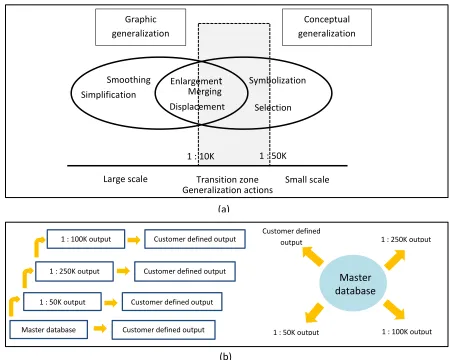
Figure 2.3 (a) Relation between graphic and conceptual generalization and (b) Ladder approach left and Star approach right. ... 17
Figure 2.4 Generalization as a sequence of modelling operations ... 18
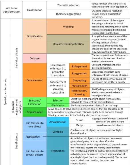
Figure 2.5 Generalization operators defined for the AGENT project simplified after Bader et al. (1999) ... 21
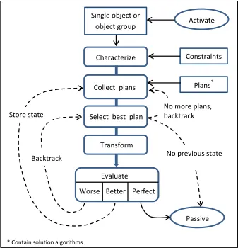
Figure 2.6 AGENT generalization procedure for a single object or a group of objects... 24
Figure 2.7 Characteristics of an MRDB - storage of multiple representations of objects (left) and linkage of corresponding objects (right). ... 26
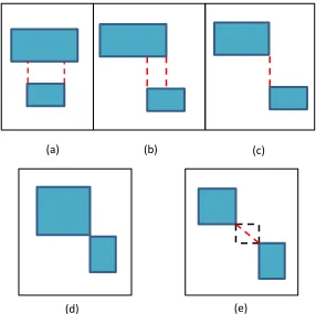
Figure 2.8 (a) A pair of buildings at total separation (b) displacement of building B1 to building B2 has created a corner touching situation and (c) rotating, aligning and merging of building B1 with building B2, has created a corner touching situation. ... 28
Figure 2.9 A pair of buildings in a cluster at different positions: (a) total overhanging (b) partial overhanging (c) almost overhanging (d) corner touching and (e) total separation. ... 28
Figure 2.10 Area aggregation based on morphological operators. ... 29
Figure 2.11 Building aggregation. ... 30
Figure 2.12 Building clustering with three steps. ... 35
Figure 2.13 Building clustering with the MST. ... 37
Figure 2.14 Hierarchical relationship of constraints for building clustering ... 40
Figure 2.15 (a) A domain (Ω) with a set of points and (b) triangulation of the points. ... 42
Figure 2.16 (a) Non-Delaunay and (b) Delaunay stable triangulation, based on Žalik (2005). ... 42
Figure 2.17 (a) A planar points and straight line edge graph G(P, E) called PSLG (b) conventional Delaunay triangulation of point set P (c) CDT of G(P, E) and (d) illustration of the modified
circumcircle criterion on the hatched triangle for the CDT. ... 45
Figure 2.18 Execution of the CNDT algorithm on a simple example. ...48
Figure 2.19 Continuation of the CNDT algorithm with splitting edges and triangles. ... 49
Figure 2.20 Recursive process of finding triangles in polygon triangulation. ... 51
Figure 2.21 CDT of a set of building objects with constraining edges is shown in solid lines while other virtual edges are shown in dashed lines. ... 52
Figure 4.1 (a) CDT with duplicate nodes of triangles hatched in grey colour and (b) Hashtable data structure to handle duplicates. ... 80
Figure 4.2 (a) CDT with a triangle comprising of duplicate nodes hatched in red colour and (b) the same hatched triangle with duplicate node IDNs generated from building number attached at three corners... 81
Figure 4.3 (a) Outer polygon and inner building polygons (triangulating features) with corner coordinates and (b) representation of the outer polygon and the two inner building polygons in ASCII format... 83
Figure 4.4 (a) Building polygons (triangulating features) with corner coordinates and (b) representation of two building polygons in ASCII format. ... 85
Figure 4.5 Constrained triangulation algorithm based on the polygon triangulation on ear-clipping by Eberly (2008). ... 90
Figure 4.6 (a) A simple data set of buildings and (b) a larger data set with buildings irregularly spaced, triangulated based on the polygon triangulation. ... 92
Figure 4.7 Building polygons with local IDNs in a single region surrounded by the road network. 93 Figure 4.8 Insertion point location: (a) inside triangle (b) outside convex hull of ΔN, (c) on an edge of an interior triangle of ΔN and (d) on an edge of a triangle bounded by convex hull to form the initial triangulation Δ’N+1.. ... 95
Figure 4.9 Swapping procedure when inserting a point p into Delaunay triangulation.... 96
Figure 4.10 Default Delaunay triangulation ... 97
Figure 4.12 Re-triangulation steps of the isolated polygons after subtraction of triangles and building polygons from the convex hull of all the site points P. ... 99 Figure 4.13: Crossing triangles to be removed in the triangulation process. ... 100 Figure 4.14 (a) Constrained triangulation with duplicate nodes of a triangle hatched in red colour (b) same triangle with duplicate node IDNs and distances of the three edges D1, D2 and D3 and (c)
array representing proximity links of both contiguous and disjoint buildings with the minimum Euclidean distance. ... 103 Figure 5.1 (a) Hierarchical structure of the road network (part) and (b) manual process of building grouping ... 112 Figure 5.2 Hierarchical relationship between the three local constraints for building grouping. ..113 Figure 5.3 Existing measures of building orientation. ... 114 Figure 5.4 Smallest minimum bounding rectangle (SMBR). ... 115 Figure 5.5 Calculation of the Hausdorff distance. ... 119 Figure 5.6 (a) DCT (b) adjacency relationship list (part) comprising of [bid_from, bid_to, proximity, orientation difference, similarity difference] and (c) MST segmentation in thick black lines with proximity as the weight. ...121 Figure 5.7 (a) 2D initial adjacency matrix based on the proximity hierarchy depending on the target map scale and (b) example of the distribution of buildings spaced at three levels - VC, M and VF. ... 122 Figure 5.8 An example of linked pairs and non-linked pairs with building IDNs in a column of the adjacency matrix. ...123 Figure 5.9 (a) Separation threshold between two buildings and (b) angle ө subtended by an arc of 0.125mm with radius r = 1m. ... 128 Figure 5.10 Automatic building clustering. Source data at the scale of 1 : 1.25K and the clusters are formed from the source data at the target map scale of 1 : 5K for the subsequent map generalization. ... 130 Figure 5.11 Automatic building clustering on the source data at the scale of 1 : 1K . ... 131 Figure 5.12 Automatic clustering results in: (a) region 1 (b) regions 14, 15 and 16 (c) regions 11, 12 and 13 and (d) region 19. ... 136
Figure 5.13 (a) Partitioned regions surrounded by the road network where inner roads are ignored
and (b) building features within each region ... 138
Figure 5.14 Automatic building clusters (yellow) in region 9 used in the clustering experiment. 147 Figure 5.15 Generation of the CNDT using buildings and roads with the enforcement of their edges as constraints within region 9 used in the clustering experiment. ... 148
Figure 5.16 Automatic building clusters (light green) in region 9 after deriving adjacency relationships between buildings, taking into account the contextual inner roads within the region. ... 149
Figure 5.17 Building clusters on synthetic data. ... 151
Figure 5.18 Concave hull generation of a concave cluster of buildings on synthetic data. ... 152
Figure 5.19 Concave hull generation of a convex cluster of buildings on synthetic data. ... 153
Figure 5.20 Shape enrichment of clusters in three regions 4, 5 and 7 (part of) surrounded by the road network. ... 155
Figure 5.21 Shape enrichment of clusters in the same three regions 4, 5 and 7 (part of) surrounded by the road network as shown in Figure 5.20 with some improved results... 158
Figure 5.22 Data enrichment workflow of creating clusters and their subsequent shape enrichment ... 162
Figure 6.1 Building at a corner. ... 171
Figure 6.2 Buildings with three neighbouring road segments around. ... 171
Figure 6.3 Different orientation of the LOBR of a building to the closest road. ... 173
Figure 6.4 LOBR of the building with two line segments connecting the centroid and midpoints of its edges. ... 174
Figure 6.5 Results of building orientation to the road on the OS MasterMap Data within a region surrounded by the roads. ... 177
Figure 6.6 Synthetic data set with its attributes at a decision point. ... 182
Figure 6.7 COBWEB clustering tree view (left) and the matrix showing cluster numbers against instances (right) of the synthetic data set in Figure 6.6. ... 184
Figure 6.8 Graphical representation of an enriched tree view with attributes, their values and
instance IDNs (class IDNs) after the analysis. ... 184
Figure 6.9 Transformation (discretization) of the attribute - neighbour - in the synthetic data set in the WEKA GUI. ... 186
Figure 6.10 Classification output of the synthetic data set: (a) output at first iteration with the first instance hypothesized to be a landmark and (b) output at third iteration with the third instance hypothesized to be a landmark. ... 187
Figure 6.11 Classification output of the synthetic data set at the third iteration with the third instance hypothesized to be a landmark. ... 189
Figure 7.1 Generating group oriented bounding rectangle (GOBR). ... 200
Figure 7.2 Building enlargement: (a) enlargement along the Y-axis (height) and (b) enlargement along the X-axis (width) to comply building edges with the minimum building length. ... 201
Figure 7.3 Example illustration of a buffer around a polygon with cap square and join style mitre. ... 203
Figure 7.4 A pair of buildings in a cluster at different positions: (a) almost overhanging, (b) corner touching and (c) total separation. ... 203
Figure 7.5 Polygon geometry shown in red colour using the dilation operation and then the erosion with iterative shrinking for exceptional cases. ... 204
Figure 7.6 Squaring of an initial amalgam of a building cluster created using a synthetic data set with ear polygons. ... 206
Figure 7.7 Creating rectangular strips required in the enlargement process. ... 211
Figure 7.8 Selection of filling rectangular strips in the enlargement process. ... 212
Figure 7.9 Possible cases of building enlargement with narrow sections. ... 213
Figure 7.10 Introduction of granular edges in the amalgam after squaring and enlargement. .... 214
Figure 7.11 Simplification of the amalgam with orthogonal sides. ... 216
Figure 7.12 Functional process of building symbolization and aggregation with orthogonal sides. ... 217
Figure 7.13 Result of buffering with same positive and negative distance: (a) source cluster and (b) buffered amalgam with the two leftmost buildings (IDNs 1 and 2) bridged together, and two other source buildings (IDNs 3 and 4) in the cluster. ... 223 Figure 7.14 DCT on the buffered amalgam ... 224 Figure 7.15 Triangles selected for bridging based on the distance threshold highlighted in yellow colour. ... 225 Figure 7.16 Results of the aggregation of building clusters with orthogonal sides on a real data set representing a region after squaring, enlargement and simplification. ... 228 Figure 7.17 Result of buffering with the same positive and negative distance: (a) source cluster with the lower building comprising of two concave corners shown circled and (b) buffered amalgam where the two concave corners are filled as a result of the buffering operation. ... 231 Figure 7.18 Result of buffering with the same positive and negative distance: (a) source cluster including a polygon with a hole and (b) buffered amalgam in a multi-polygon with a filling bridge between the two leftmost buildings and the preserved hole of the rightmost building in the source cluster in (a). ... 231 Figure 7.19 DCT on the buffered amalgam. ... 232 Figure 7.20 Possible cases of bridging a pair of buildings. ... 234 Figure 7.21 Dealing with polygon holes after aggregation of buildings with non -orthogonal sides. ... 237 Figure 7.22 Functional process of building aggregation with non-orthogonal sides... 238 Figure 7.23 Results of the aggregation of non-orthogonal shaped clusters comprising of buildings with non-orthogonal sides and/or significant orientation difference. ... 241 Figure 7.24 Results of the generalized amalgams with the improved concave hull algorithm... 242 Figure 8.1 Results of the CNDT with the edge constraints. ... 247 Figure 8.2 Results of clustering: (a) incorrect clustering due to topologically incorrect triangulation (highlighted in yellow colour) and (b) correct clustering after the fix of CNDT with the edge constraints. ... 248 Figure 8.3 Results of building orientation to the closest road. ... 249 Figure 8.4 Results of building orientation to the closest road after fixing the exceptions. ... 250
Figure 8.5 Results of building orientation to the closest road, located at corners... 251 Figure 8.6 Enlargement results after squaring with a distance 5m. ... 251 Figure 8.7 Simplification of a building with the OpenCarto edge deletion algorithm. ... 254 Figure 8.8 Location map of the London Boroughs of Newham and Tower Hamlets (hatched).... 256 Figure 8.9 Newham test area: (a) road network with the classification of roads comprising of minor roads, private roads and alleys and (b) chosen regions (area partitions) for data processing during the focus map generation. ... 257 Figure 8.10 Source map of Newham test area at the scale of 1 : 8K. ... 258 Figure 8.11 Generalized building amalgams at the target scale of 1 : 8K to be used as the background on the focus map, derived from the source data at the scale of 1 : 1.25K in Newham area (part of). ... 259 Figure 8.12 Focus map with salient building landmarks highlighted with the graphical variable - colour - portrayed in the original shape on the coarse background of the generalized buildings at the target scale of 1 : 8K, derived from the source data at the scale of 1 : 1.25K in Newham area (part of). …... 260 Figure 8.13 Tower Hamlets test area: (a) road network with the classification of roads comprising of minor roads, private roads and alleys and (b) chosen regions (area partitions) for data processing during the focus map generation... 261 Figure 8.14 Source map of Tower Hamlets test area at the scale of 1 : 8K. ... 262 Figure 8.15 Generalized building amalgams at the target scale of 1 : 8K to be used as background on the focus map, derived from the source data at the scale of 1 : 1.25K in Tower Hamlets area (part of). ... 263 Figure 8.16 Focus map with salient building landmarks highlighted with graphical variable - colour - portrayed in the original shape on the coarse background of the generalized amalgams of buildings at the target scale of 1 : 8K, derived from the source data at the scale of 1 : 1.25K in Tower Hamlets area (part of)... 264 Figure 8.17 Generalization results of clusters of orthogonal shape: (a) three source clusters highlighted in yellow colour (b) generalized amalgams with a distance of 4m (c) generalized amalgams in the ArcGIS software with a distance of 4m and (d) generalized amalgams in the ArcGIS software with a distance of 16m. ...268
Figure 8.18 Generalization results of clusters of non-orthogonal shape with the research tool. . 269 Figure 8.19 Generalization results of clusters of non-orthogonal shape with the ArcGIS software. ... 270 Figure 8.20 Comparison of amalgams of the non-orthogonal shaped cluster depicted in Figure 8.19(a) above. ... 271 Figure 8.21 Generalization results of clusters of orthogonal shape: (a) two source clusters highlighted in yellow colour (b) amalgams with an aggregation, exaggeration and simplification distance of 4m with the research tool (c) amalgams in (b) overlaid with source clusters in (a), and (d) amalgams after simplification with a tolerance of 4m using the ArcGIS software. ... 272 Figure 8.22 Generalization results of a cluster of non-orthogonal shape: (a) source cluster highlighted in yellow colour (b) amalgam with an aggregation distance of 4m and a space triangle edge threshold of 4m (c) amalgam before simplification with the two thresholds with a value of 8m (d) amalgam after simplification with 4m tolerance with the research tool (e) amalgam before simplification with a distance of 8m and (f) amalgam after simplification with a tolerance of 4m with the ArcGIS software. ... 273 Figure 8.23 Generalization results of a cluster of non-orthogonal shape: (a) two source clusters highlighted in yellow colour (b) amalgams with an aggregation distance of 4m and a space triangle edge threshold of 4m with the research tool and (c) amalgams with an aggregation distance of 4m with the ArcGIS software, no simplification applied in both cases. ... 275 Figure 8.24 (a) Salient landmarks (highlighted in yellow colour) derived from region 3 of Newham area (see Figure 8.9), delineated in blue and (b) salient landmarks (highlighted in yellow colour) derived in sub-regions 3A and 3B of the main region 3, applying the J48 implementation in each sub-region separately. ... 277 Figure 8.25 Landmark saliency results (highlighted in yellow colour) of region 5 of Newham area: (a) results by the J48 implementation and (b) results by the framework of Raubal and Winter (2002) . ... 284 Figure 8.26 Landmark saliency results (highlighted in yellow colour) of region 1 of Tower Hamlets area: (a) results by the J48 implementation and (b) results by the framework of Raubal and Winter (2002) . ... 284
Figure 8.27 Landmark saliency results (highlighted in yellow colour) of region 5 of Newham area: (a) results by the J48 implementation and (b) results by the new method on the MAD developed in
this research... 290
Figure 8.28 Landmark saliency results (highlighted in yellow colour) of region 1 of Tower Hamlets area: (a) results by the J48 implementation and (b) results by the new method on the MAD developed in this research. ... 291
Figure 8.29 Focus map of Newham area with the insets A, B, C and D of the specific locations considered in the validation of the landmark saliency. ... 292
Figure 8.30 Salient landmark visualization on Swete Street ... 293
Figure 8.31 Salient landmark visualization on Ballam Street and Dongola Road West. ... 294
Figure 8.32 Salient landmark visualization on Whitwell Road and Grant Street. ... 295
Figure 8.33 Salient landmark visualization on Barking Road. ... 296
Figure 8.34 Focus map of Tower Hamlets area with the insets A, B and C of the specific locations considered in the validation of the landmark saliency. ... 300
Figure 8.35 Salient landmark visualization on Goldsmith’s Row... 301
Figure 8.36 Salient landmark visualisation on St. Peter’s Close. ... 302
Figure 8.37 Salient landmark visualisation on Centre Street ... 303
Figure 8.38 Google street view of high-rise buildings with the same shape and the height visualized from the middle of the Centre Street. ... 306
Figure 8.39 Focus map of Tower Hamlets area with the decision point circled, and the regions (1 to 5) used in deriving landmark saliency. ... 307
Figure 8.40 Evaluation of salient landmarks at a decision point with the J48 implementation: (a) Salient landmarks falling within the buffer of 50m, derived from each region separately (regions 2, 3, 4 and 5 in Figure 8.39 and (b) salient landmarks derived from all the buildings within the same buffer at the decision point during focus map generation in Tower Hamlets area. ... 308
Figure 8.41 Evaluation of the landmark saliency at a decision point in Tower Hamlets area: (a) all the buildings around the decision point within a radius of 50m (b) salient landmarks chosen by the J48 implementation and (c) salient landmarks chosen by the implementation of the framework of Raubal and Winter (2002) from the buildings with a total significance >= 0.75. ... 309
Figure 8.42 Evaluation of the landmark saliency at a decision point in Tower Hamlets area with all the buildings around the decision point within a radius of 50m: (a) salient landmarks chosen by the framework of Raubal and Winter (2002) from the buildings with a total significance >= 0.75 and (b) salient landmarks chosen by the new method on the MAD from the buildings with a total significance >= 1 and the significance contribution from two or more significance measures. .... 312 Figure 8.43 Focus map with salient building landmarks highlighted with graphical variable - colour - portrayed in the original shape on the coarse background of the generalized buildings at the target scale of 1 : 8K, derived from the source data at the scale of 1 : 1.25K in Newham area (part of). ... 321 Figure 8.44 Focus map with salient building landmarks highlighted with graphical variable - colour - portrayed in the original shape on the coarse background of the generalized amalgams of buildings at the target scale of 1 : 8K, derived from the source data at the scale of 1 : 1.25K in Tower Hamlets area (part of)... 322 Figure A.1 (a) Dialogue menu with the coordinate values of the MBB of the building data set retrieved automatically for generating outer polygon of the input data structure and (b) input building geometries in ASCII format where polygon IDN of the outer polygon (MBB) is assigned -1. ... 350 Figure A.2 (a) Dialogue menu to extract and save building polygon geometries in ASCII format and (b) extracted building outer polygon geometries with respective building IDNs. ... 351 Figure B.1 (a) CDT output with rectangular buildings outlined in red colour and their IDNs on the GUI and (b) adjacency links between buildings where Polygon IDN 1 is the IDN of the outer polygon. ... 352 Figure B.2 (a) CNDT output and (b) output on polygon triangulation based algorithm with the edges of building polygons set as constraints, both implemented on the same GUI. ... 353 Figure B.3 GUI for spatial clustering of building polygon geometries in the data enrichment process with the use of constrained algorithm on Delaunay triangulation. ... 354 Figure B.4 Distance weighted initial MST in thick black lines used for clustering of building geometries. ... 355 Figure B.5 UI for matching automatic clustering results with that of manual clustering by the subjects in both expert and lay groups. ... 356
Figure B.6 GUI for spatial clustering of building polygon geometries with the consideration of the
contextual features (roads in black colour) using the CNDT with edge constraints... 357
Figure B.7 Cluster shape enrichment of building clusters. ... 358
Figure B.8 Generalization GUI for building geometries. ... 359
Figure C.1 Contribution of an edge of a building to a candidate orientation αi on modulo π/2. .. 362
Figure C.2 Simplification of shorter edges. ... 363
Figure D.1 Source map at 1 : 4K (left) and the target map reduced and printed at 1 : 10K (right). ... 364
Figure D.2 Regions surrounded by the road network. ... 365
Figure D.3 Building features in each region depicted by a unique colour. ... 366
Figure D.4 Manual clustering output of a subject from the expert group... 368
Figure D.5 Manual clustering output of a subject from the lay group. ... 369
Figure F.1 Sensitivity analysis workflow in the WEKA GUI. ... 400
Figure F.2 Output of the sensitivity analysis in the WEKA GUI. ... 401
Figure F.3 Attribute transformation with the unsupervised discretization. ... 402
Figure F.4 Data mining UI for extracting the salient landmarks using the algorithms - CobWeb, ID3 and J48 - implemented with the open source WEKA Java APIs. ... 403
Figure F.5 User interface for the salient landmark evaluation based on the two frameworks of (a) Raubal and Winter (2002) and (b) Nothegger, Winter and Raubal (2004), and the method on the MAD developed in this research. ... 405
List of Tables
Table 4.1 Results of the CDT based on the sweep line algorithm by Domiter and Žalik (2008) with
different data sets ... 84 Table 4.2 Results of the CNDT based on the incremental algorithm by Ruppert (1995). ... 88 Table 4.3 Results of the constrained triangulation developed in this research based on the polygon triangulation algorithm by Eberly (2008) on the source data. ... 91 Table 4.4 Results of the constrained triangulation developed in this research based on the Delaunay triangulation with the recursive edge-flipping technique (Berg et al., 2008) using the incremental method. ... 101 Table 4.5 Computation times to generate triangulation and neighbourhood relations. ... 104 Table 4.6 Validation of the constrained triangulation developed using the edge deletion method (Shewchuk, 1999). ... 105 Table 4.7 Different triangulation types implemented and compared. ... 108 Table 5.1 Typical examples of the orientation difference between a rectangular pair of buildings based on the wall orientation algorithm by Duchêne et al. (2003) ... 116 Table 5.2 Main polygon building clustering algorithm with the contributing algorithms ... 132 Table 5.3 Summary of the clustering results of the expert group derived from the cluster data given in Appendix D.6 in each of the twenty two regions compared with automatic clustering results. ... 134 Table 5.4 Summary of the clustering results of the lay group derived from the cluster data given in Appendix D.6 in each of the twenty two regions compared with automatic clustering results. ... 135 Table 5.5 Summary of the results in identifying the medium distance range clusters for the hierarchical application of the Gestalt constraints - orientation and similarity difference - by the expert and the lay groups, derived from the cluster data given in Appendix D.6. ... 137 Table 5.6 Summary of the results of percentages of the subjects in both groups identifying clusters with a misclassification, derived from the cluster data given in Appendix D.6. ... 139 Table 5.7 Evaluation of the automatic clustering method by the expert and the lay groups. ... 140
Table 5.8 Evaluation of the use of threshold values of the Gestalt factors - proximity, orientation and similarity in the automatic clustering method by the expert and the lay groups. ... 141 Table 5.9 Evaluation of the comparison of manual clustering approach with the automatic clustering by the expert and the lay groups. ... 142 Table 5.10 Evaluation of the adaptation of manual clustering process by the expert and the lay groups. ... 143 Table 5.11 Summary of the answers to the Question 3(b) of the questionnaire in Appendix D.7 ... 143 Table 5.12 Summary of the answers to the Question 4(b) of the questionnaire in Appendix D.7 ... 144 Table 5.13 Summary of the answers to the Question 6(b) of the questionnaire in Appendix D.7 ... 145 Table 5.14 Summary of the answers to the Question 9(b) of the questionnaire in Appendix D.7 ... 145 Table 5.15 Enlarged view of the clusters delineated in Figures 5.20 and 5.21 for the clear view of the orientation difference... 159 Table 5.16 Cluster shape enrichment algorithm with the contributing algorithms. ... 161 Table 6.1 Description of attributes considered to derive salient landmarks in the data mining process. ... 166 Table 6.2 Building categories and their priority rankings. ... 179 Table 6.3 Instances with attributes chosen after the sensitivity analysis on the synthetic data set where the attribute lmark is the classifier used as a dependent variable. ... 187 Table 6.4 Results of the COBWEB clustering on the top level of the tree. ... 192 Table 6.5 Results of the COBWEB clustering using the top two levels of the tree. ... 192 Table 6.6 Results of the ID3 classification ... 193 Table 6.7 Results of the J48 classification on the top level of the tree. ... 194 Table 6.8 Results of the J48 classification using the top two levels of the tree. ... 194
Table 6.9 Comparison of the results of the three data mining algorithms using the top level and the very next lower level (1st and 2nd physical levels) of the output trees on a building data set spread
over a region enclosed by roads. ... 197 Table 7.1 Test results of the building aggregation algorithm with dilation and erosion followed by squaring the sides of the amalgam. ... 208 Table 7.2 Test results of the building aggregation algorithm with concave hull generation followed by squaring the sides of the amalgam. ... 209 Table 7.3 Test results I of building aggregation algorithm with orthogonal sides... 218 Table 7.4 Test results II of the building aggregation algorithm with orthogonal sides. ... 220 Table 7.5 Results of further testing of the building aggregation algorithm with orthogonal sides using an exceptional synthetic data set. ... 221 Table 7.6 Results of the aggregation of building clusters with orthogonal sides on the synthetic data used in Table 7.5 with some exceptional building configuration. ... 227 Table 7.7 Building cluster aggregation algorithm with orthogonal sides, including contributing algorithms. ... 229 Table 7.8 Pairing algorithm of adjacent triangles. ... 236 Table 7.9 Results of aggregation of building clusters with non-orthogonal sides on the synthetic data with some exceptional building configuration. ... 240 Table 7.10 Building cluster aggregation algorithm with non-orthogonal sides, including contributing algorithms... 243 Table 8.1 Evaluation of the generalization constraints on amalgams of Newham data. ... 271 Table 8.2 Evaluation of the generalization constraints on amalgams of Tower Hamlets data. ... 276 Table 8.3: Method of calculating the overall significance score of each building using individual significance value of each attribute based on the framework by Nothegger, Winter and Raubal (2004). ... 279 Table 8.4 Deriving a total significance score for a particular building by the method of Raubal and Winter (2002). ... 281 Table 8.5 Evaluation of landmark saliency of the focus map with the framework of Raubal and Winter (2002) in the regions depicted in Figure 8.9, page 257 of Newham area. ... 282
Table 8.6 Evaluation of landmark saliency of the focus map with the framework of Raubal and Winter (2002) in the regions depicted in Figure 8.13, page 261 of Tower Hamlets area. ... 282 Table 8.7 Attributes and their transformed values to be compatible with the new landmark saliency measure. ... 287 Table 8.8 Deriving a total significance measure for landmark saliency for a building to be applied to the new method based on the MAD. ... 288 Table 8.9 Evaluation of landmark saliency with the new method developed on the MAD in the Newham data set... 289 Table 8.10 Evaluation of landmark saliency with the new method developed on the MAD in Tower Hamlets data set. ... 289 Table 8.11 Landmark significance together with attributes and their values of the four chosen salient landmarks with the J48 implementation. ... 310 Table 8.12 Landmark significance together with attributes and their values of the four chosen salient landmarks with a total significance >= 0.75 based on the framework by Raubal and Winter (2002). ... 310 Table 8.13 Comparison of landmark significance together with individual significance scores of each measure of the most prominent salient landmarks chosen based on the framework by Raubal and Winter (2002) and the new method based on the MAD. ... 312 Table D.1 Results of the expert group in each partitioned region. ... 370 Table D.2 Results of the lay group in each partitioned region. ... 381 Table F.1 Enriched test data (part of) of a region surrounded by the road network. Data source: OS MasterMap. ... 404 Table F.2 Results of the salient landmarks at a decision point. ... 406
List of Abbreviations
AGENT: Automatic GENaralization New Technology API: Application Programming Interface
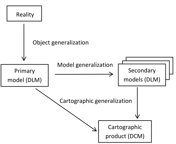
CDT: Constrained Delaunay Triangulation CNDT: Conforming Delaunay Triangulation DCM: Digital Cartographic Model
DCT: Delaunay Constrained Triangulation DEM: Digital Elevation Model
DF: Distance Factor
DLM: Digital Landscape Model DHD: Discrete Hausdorff Distance
ESRI: Environmental System Research Institute GIS: Geographic Information System
GPS: Global Positioning System GSP: Good Sub-Polygon
GOBR: Group Oriented Bounding Rectangle GUI: Graphical User Interface
HD: Hausdorff Distance
ICA: International Cartographic Association IDN: Identification Number
JCS: Java Conflation Suite JTS: Java Topology Suite
KDD: Knowledge Discovery in Database LBS: Location Based Services
LOBR: Locally Oriented Bounding Rectangle MAD: Median Absolute Deviation
MBB: Minimum Bounding Box MBR: Minimum Bounding Rectangle MRDB: Multiple Representation Database
MRDBMS: Multiple Representation Database Management System MSL: Mean Sea Level
MST: Minimum Spanning Tree NMA: National Mapping Authority OGC: Open Geospatial Consortium OS: Ordnance Survey
POI: Points of Interest
PSLG: Planar Straight Line Graph RNG: Relative Neighbourhood Graph
SMBR: Smallest Minimum Bounding Rectangle STR: Sort-Tile-Recursive
2D: Two-Dimensional 3D: Three-Dimensional UI: User Interface
Acknowledgements
First and foremost, I want to express my deepest and sincere gratitude to my main supervisor and the director of studies Professor Allan J. Brimicombe for his continuing guidance, advice and encouragements throughout the duration of my study. I had the opportunity to learn a lot in the field of research through his vast experience as a cross-disciplinary researcher. I would like to thank Dr. Yang Li, my second supervisor for his constructive criticisms, suggestions and valuable feedback that contributed to the successful completion of the research.
I take this opportunity to offer my special appreciation to all those who provided valuable support in sharing their knowledge and ideas to solve the issues I encountered in my work through the open source user forums. Special thanks should go to Dr. Martin Davis - the developer of the Java topology suite (JTS): a two-dimensional (2D) spatial predicates library, Mr. Micheal Bedward – the geographical information system developer of OpenJump and Dr. Stefan Steinger - Postdoctoral Research Associate from the University
of Calgary and Pontifica Universidad Católica de Chile - for providing me with open source
libraries and useful resources in the area of the research.
I extend my gratitude to the school of Architecture, Computing and Engineering, and the Graduate school for the support provided to carry out the research, ensuring an excellent atmosphere from the beginning to the end.
My sincere thanks should also be extended to the Ordnance Survey of the United Kingdom for the production of highly detailed Ordnance Survey MasterMap data that I used in my work for conducting the research.
This acknowledgement would not have been complete without mentioning the name of the National Mapping Authority in Sri Lanka for setting an encouraging platform to peruse higher studies and providing useful resources for conducting the research.
Dedication
This dissertation is dedicated to my loving family for the constant support and encouragement that has made this work possible. Finally, I dedicate this work in memory of my father who always encouraged me to the pursuit of academic excellence.
Chapter 1 Introduction
This chapter provides the motivation for taking up this research where it discusses the background of wayfinding and broad aspirations of what is to be achieved through this research.
1.1 Research motivation
The use of geographic information through mobile applications has been rapidly increasing and enabling users to view their current position in the context of the neighbouring environment through the advancement of technologies such as Global Positioning System (GPS) and ubiquitous computing Internet technologies, along with the availability of mobile devices. Thus, one of the major challenges facing the national mapping authorities (NMAs) across the world is the development of maps that are more helpful and attractive to be used in mobile applications such as in wayfinding. This necessity is emphasised in the usability evaluation of topographic maps for mobile devices where users need more meaningful map entities in topographic maps that should be adapted, according to their context of use according to Nivala et al. (2003), since cartographic presentation and symbology in traditional topographic maps are not designed for wayfinding applications.
Wayfinding is the process by which human beings orient themselves and navigate through space. According to Allen (1999) wayfinding by human beings can be mainly for three purposes: (a) travel with a goal of reaching a familiar destination (b) exploratory travel with the view of returning to a familiar point of origin and (c) travel with the goal of reaching a novel destination. Therefore, it is evident that wayfinding involves direct interaction between the traveller and the environment. Human beings use various spatial, cognitive and behavioural abilities to find their way through the environment, gaining environmental information or spatial knowledge about the environment (Raubal and Winter, 2002; Lloyd, 1989; Gopal and Smith, 1990; Cornell, Sorenson and Mio, 2003; Brimicombe and Li, 2010). According to Kuipers (1978), people acquire spatial knowledge in positioning through route descriptions, topological relations of the road network and
the orientation of objects in the environment. Research in spatial cognition has shown that maps are a vital means of providing spatial knowledge to assist travellers acquire route information to reach their destination without trouble (MacEachren, 1995; Kray et al., 2003; Elias and Paelke, 2008).
Further experiments conducted by Denis et al. (1999), Freksa et al. (1999), Tversky and Lee (1999) and Montello, Michon and Denis (2001) have shown that pedestrians perceive landmarks as a useful part of route information in wayfinding. Lynch (1960) describes landmarks as defined physical objects external to the observer and that are used as a point of reference to make one orient oneself. According to Golledge (1999), landmarks are physically defined objects that stand out from the surroundings and help locate geographic position. More meaningfully, landmarks are cognitively distinct from other elements in spatial memory and central to the nature and organisation of spatial representation (Presson and Montello, 1988).
Thus, including supplemental landmarks could make travellers much more confident and comfortable when experiencing a new environment irrespective of the navigation aids whether they be a traditional paper street map or a vehicle navigation system (Deakin, 1996). However, according to Deakin (1996), one of the reasons for the non-inclusion of supplemental landmarks on street maps arises from the difficulty of selecting such landmarks that are salient based on a standard methodology and criteria. Another issue is the limited map space to incorporate landmarks, which requires the application of map generalization techniques to reduce map details to accommodate space. Although current navigation systems utilise visual representation in addition to positioning and routing functionality to convey navigational information to the users, landmarks are still missing in spatial data sets in such applications due to aforesaid limitations. However, various approaches by Raubal and Winter (2002), Elias (2003), Elias and Brenner (2005) and Elias, Hampe and Sester (2005) have been attempted to derive salient landmarks from spatial data sets to improve navigation aids. Evaluation of such methods in terms of geometrical, spatial and semantic characteristics of such landmarks for the effective integration of them into both static maps and mobile maps (maps that can be accessed wirelessly to use
in mobile situations (Meng and Reichenbacher, 2005) for wayfinding) has not been investigated yet. Further, due to the technical limitations such as processing power, memory, resolution and small screen size in mobile devices, the general cartographic rules in applying colours, symbology and feature representation in map production could not be used in mobile mapping. To this effect, some research has discussed the cartographic repercussions of small displays (Gartner and Uhlirz, 2001; Radoczky and Gartner, 2005; Elias, Hampe and Sester, 2005).
Therefore, it is understood that there is a significant difference between a traditional topographic map and a map designed for mobile navigation especially considering the limitations discussed above. Another important factor in designing a mobile map is to enable users to engage in the wayfinding task by presenting him/her an egocentric map view which is more a technique of representing geographic information in relation to a user’s position (Meng, 2005). This not only keeps users focused on the task of interest without distracting him/her from other external interferences in the environment, but also improves his/her cognitive capability of understanding the immediate surroundings of the navigation route in a manner which is not the same as gathering spatial knowledge by reading a traditional topographic map. In a traditional topographic map, a uniform visual balance of details is maintained with an allocentric view (viewing location of one object in relation to other objects) throughout the map at a uniform scale. This emphasises that mobile applications for wayfinding should allow users to bring to their attention the areas of interest rather than searching for important locations and prominent features, reading through the whole map as is the case in retrieving information from a traditional analogue topographic map.
Thus, the NMAs should aim to produce customer-oriented mobile maps, incorporating important landmarks that are more useful and attractive to users in finding points of interest with the minimum effort using cartographic visualisation techniques discussed above rather than necessarily giving priority to producing conventional topographic map series along their production lines. Being a surveyor by profession in the NMA of Sri Lanka, having read Master of Science Degree in Geoinformatics at the Faculty of Geo-information
Science and Earth Observation (ITC) of the University of Twente, the Netherlands, with a specialisation in multiple representation visualisation of topographic features of the same phenomena, I have been persuaded to take up this research which is oriented towards investigating the automatic processes of developing visually appealing maps primarily designed for wayfinding users to bring their immediate focus to the area of interest with highly detailed, prominent features and leaving all other information in the peripheral areas with the coarse background information.
1.2 Background
With the growth of ubiquitous computing through the emergence of mobile devices and distributed applications over the Internet, personalisation is leaving the desktop domain (Günter, 1991; Zipf and Jöst, 2006). A widespread availability of mobile devices and the distributed applications via wireless access have allowed people to access maps in mobile situations personally rather than using fixed line, personal computer based web maps. Particularly, ubiquitous computing has brought location based services (LBS) into existence with a variety of spatial applications. LBS are regarded as services that deliver data and information customised to the current or some projected location and context of the user (Brimicombe and Li, 2006). As one of the principal and useful applications in LBS, using lightweight mobile devices to point the location on Earth has been popular with the rapid development of geographic information system (GIS), GPS, radio frequency identification and various other location sensing technologies with varying degrees of accuracy (Jiang and Yao, 2006). According to Reichenbacher (2003), a mobile user can perform various tasks in relation to geoinformation in the real world: locating, navigating, searching, identifying and checking. Maps containing these geoinformation can either be stored in the mobile device or retrieved online. Locating is related to the question “where am I?” or “where is X?”. Navigating involves wayfinding either from the user’s current position to a given position or object or between any specified objects/positions independent of the user’s current location. Searching deals with finding objects or people located from the user’s current position. Identifying relates to the recognition of objects in relation to the other objects in the vicinity. Finally checking relates to an event task for
finding information about what happens at a given place. As a result of the capabilities of such spatially related tasks, wayfinding has become one of the most popular applications for small electronic devices such as smartphones. Further, in contrast to in-vehicle navigation systems (such as SatNavs), the increasing demand for the use of mobile phones has also brought pedestrian wayfinding to the fore (Elias, Hampe and Sester, 2005). Such pedestrian wayfinding systems depend heavily on maps to convey wayfinding information to the users in addition to positioning and routing functionality (Elias and Paelke, 2008). However, different visualisation techniques such as changing the opacity/colours of features (Reichenbacher, 2004, 2005; Figure 1.1 below) and application of the variable scale object representation techniques (Fairbairn and Taylor, 1995) have been attempted to improve the egocentric map. In addition to the technique of visualising multiple representations of data at different scales (Elias, Hampe and Sester, 2005) based on map generalization, that is, the reduction of details of a source map at a larger scale to produce a target map at a smaller scale to accommodate smaller map space. Further, a mobile map should have a task-based representation, concentrating on rich details in the area of interest while representing coarse details in the peripheral area rather than an exploratory instrument like a traditional topographic map with uniformly rich detail to gain an idea of the entire area of the map (Meng, 2005). This emphasises that a mobile map should represent highly selective information in accordance with the purpose of use (user context and objectives). Due to specific needs and technical limitations of the wayfinding systems, a relatively new concept called adaptation has been introduced in mobile geographic information applications (Zipf and Jöst, 2006). The two most important factors for adaptation are (a) the user’s objectives and (b) the context in the representation of the current situation of the immediate navigation environment. The aforesaid selective information in the immediate navigation environment should include salient landmarks as described in Section 1.1 for users to aid navigation. According to the study conducted by Lovelace, Hegarty and Montello (1999), most frequently used landmarks in finding route directions in unfamiliar environments are point landmarks (at decision points) and on-route landmarks (along the path). In addition, two other types of landmarks, distinguished by Lovelace, Hegarty and Montello (1999), are potential choice
point landmarks (street intersections) and off-route landmarks (distant but visible from the route). According to Deakin (1996), potential choice point landmarks are not distinct in an urban environment. Also, off-route landmarks are only used in navigation by a novice for overall guidance according to Lynch (1960). Further, it has been found that about 50% of all the landmarks in wayfinding instructions are buildings according to a study conducted by Elias and Paelke (2008). Therefore, a wayfinding application heavily relies on the identification of salient buildings at decision points (choice point) and along the path (on-route) of navigation.
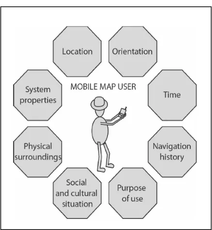
From the definition of LBS according to Brimicombe and Li (2006), it is understood that the LBS mainly consist of a system (hardware and software), user, location and context (environment). These components play a significant role in LBS applications. A number of models of these components in LBS have been presented in the literature (Sarjakoski and Nivala, 2005; Jiang and Yao, 2006; Li, 2006). According to Sarjakoski and Nivala (2005), when a mobile map in LBS is used in the field, a user has to deal with different contexts in the surrounding environment depending on the type of application (Figure 1.2).
Figure 1.1 (a) Mobile map with symbols represented by relevance values with different opacities, from Reichenbacher (2005) and (b) traditional cartographic map, from Bard (2003).
(a) (b)
Location deals with the real time information about a wayfinder’s current position on the mobile map which cannot be retrieved from a traditional hardcopy map. Wayfinding efficiency and effectiveness has a high dependency on system properties of the mobile device in terms of screen size, resolution, memory capacity and processing speed. The mobile map created should fit the situation and the purpose so that depending on the user requirement, different specific map views should be able to be generated (e.g. during daylight on a sunny day a mobile map with coloured landmarks is more useful than at night time). Also during wayfinding, depending on the time of the day, points of interest (POI) along the route may differ considerably. Another important factor in the context is the physical surroundings of the user. For example, screen display colour and brightness should adapt to the light of the physical surroundings irrespective of daylight or night and the environmental condition (a sunny day or rainy day). Further, the loss of orientation in an underground environment and disruptions, such as busyness of people during peak times, to navigation in an urban environment are some other impediments in physical surroundings. The observer’s viewpoint is also an important factor to be considered
Figure 1.2 The surrounding context of a mobile map user, from Sarjakoski and Nivala (2005).
together with the route selection based on the topography of the area of navigation. It is also important to a user to retrieve the navigation history and the planned route in some situations. Orientation is considered where the mobile map should be displayed in the right position with respect to the user’s line of sight and the direction of movement. Usage situations of mobile maps may also vary with a user’s social and cultural settings (Sarjakoski and Nivala, 2005). In addition to the purpose of use, one of the most challenging contexts to handle is the characteristics of the user him/herself. The reason is that the physical, cognitive, perceptual abilities and the personality of the user will have a considerable effect on their wayfinding scenario. However, the main aspiration of this research is towards improving the context with more emphasis on the enrichment of salient landmarks and enhancement of visual representation by way of investigating the processes to generate a focus map view (see Figure 2.1 in Section 2.1 for a variable scale focus map) using multiple representations of spatial data. It will also help NMAs produce the topographical maps and the task-oriented wayfinding maps with the inclusion of salient landmarks using a methodical and systematic approach which is still lacking in commercial navigation data sets (Elias and Paelke, 2008) and current map production at NMAs.
1.3 Outline of the thesis
Following this introductory chapter, this thesis is organised into nine chapters, and they are briefly described as follows:
Chapter 2 describes the research context. It first introduces focus maps and then presents a review of the related work in each field involved in generating focus maps. Then the overall objective is defined and research questions are formulated.
Chapter 3 presents the methodology as to how it is proposed to achieve the overall objective through answering the research questions formulated in the previous chapter. Chapter 4 describes the testing and evaluation of existing algorithms so as to develop and implement a new constrained triangulation spatial data structure to derive explicit neighbourhood relations between polygon geometries.
Chapter 5 describes how two new data enrichment algorithms: (a) spatial clustering of building polygons and (b) shape enrichment of such clusters are developed and implemented through testing, evaluating and modifying existing algorithms to be used in subsequent automatic map generalization.
Chapter 6 describes how new algorithms and methods are developed to enrich attributes that are required to derive landmark saliency of building features stored in a spatial database in the first part. In the second part, it further describes how the existing decision tree algorithms used in data mining are tested, modified and evaluated to derive the salient building landmarks with the enriched attributes during the first phase.
Chapter 7 describes how four different aggregation algorithms based on cluster characteristics enriched during the data enrichment process, are developed and implemented through testing, evaluating and modifying existing algorithms to be used in the automatic generalization of building polygons to generate a coarse background in focus maps.
Chapter 8 illustrates the results of focus map generation together with their external validation in the areas of automatic map generalization and data mining for deriving landmark saliency using the two test data sets chosen from Newham area and Tower Hamlets area of London, United Kingdom. Then it critically discusses what has been done in each area involved in generating focus maps in relation to the related work.
Chapter 9 is the conclusions where the results and the answers to the research questions are reaffirmed. Then it describes the significance of the work done in this research. Finally, it provides an outlook of the areas for future research.
Chapter 2 Research context
This chapter first introduces focus maps and then presents a critical review of related work in each area involved in generating focus maps for pedestrian wayfinding, which provides the basis for identifying the problem scope to formulate research questions. In a focus map, the user’s attention is drawn to a specific area or location with cartographic representation techniques by way of emphasising salient features. In this research on generate focus maps, four specific areas are taken into account: Delaunay triangulation data structure, data enrichment, automatic map generalization and data mining under knowledge discovery in spatial databases. These areas serve as a basis to design, implement, test and evaluate methods for generating focus maps. Delaunay triangulation will be used to get the adjacency relationships between polygonal spatial features. Data enrichment is for extracting hidden information from the spatial databases to be utilised in subsequent automatic map generalization and data mining processes. Next the main technique used to generate focus maps is the automatic map generalization. Finally, in order to retrieve salient landmarks to be incorporated into focus maps, data mining techniques are used in the knowledge discovery process.
2.1 Focus maps
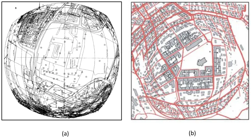
Fairbairn and Taylor (1995) have discussed methods to derive variable scale maps that are another form of focus maps based on a space-directed transformation technique (Bereuter and Weibel, 2010) in which map objects are moved apart to reduce conflicts by transforming the map space. In this process, the scale constantly decreases from the centre towards the edge of the map (Figure 2.1(a)). Further work on generating variable- scale maps has been carried out by Harrie, Sarjakoski and Letho (2002). In their approach the scale is kept constant within a circular cap based on the distance from the centre of the map while the scale of features outside the circular cap constantly decreases towards the edge of the map (Figure 2.1(b). In both approaches, details have been reduced to avoid compressed data at the edge of the maps based on map generalization before applying variable scales. Fairbairn and Taylor (1995) have applied the variable scale
approach on two data sets where data at the centre represent large scale data while the data at the edge of the map represent small scale data. Harrie, Sarjakoski and Letho (2002) have chosen a large scale data set at the centre within the circular cap while data outside the circulars cap are generalized with selection and simplification of details followed by applying a variable scale technique.
[image:40.612.123.549.183.415.2]A major characteristic of a variable scale map in wayfinding is to emphasise data in large scale at the region of interest to the user while the data in the peripheral area are represented at decreasing scales as distances increase from the centre of the area of interest. However, since the scale throughout the map is not uniform, features get cluttered towards the edge of the map even if the map generalization technique is applied to reduce details. Thus, the application of variable scale does not necessarily make the map more legible. Furthermore, the variable scale map is not visually attractive and lacks spatial fidelity because of the distortions. The evaluation of perceptual and cognitive validity of the variable scale approach in mobile map representation has not been tested.
Figure 2.1 Focus maps represented with variable scales: (a) scale radially decreases constantly from the centre of the map, from Fairbairn and Taylor (1995) and (b) scale within a circular cap based on a distance from the centre is uniform while the scale outside the area of circular cap radially constantly decreases, from Harrie, Sarjakoski and Letho (2002).
(a) (b)
To overcome the issues in distortions on variable scale maps, Rappo in 2003 as cited by Reichenbacher (2004), has used a new technique of generalization called radial generalization where the details of the map are radially generalized from the user’s position towards the edge of the map.
Zipf and Richter (2002) have applied the focus map technique to emphasise the region of interest of the user according to their current task of wayfinding by enhancing the visualisation of landmarks by the assignment of colours and an object-directed transformation technique (Bereuter and Weibel, 2010). When the object-directed transformation is applied, it is the objects in the map that are modified using map generalization operations without changing the metric properties of the underlying map space. The same concept has been extended by Neis and Zipf (2008) to represent routes with 3D landmarks (buildings) using Open Geospatial Consortium (OGC) web service standards.Reichenbacher (2005), citing his own work on the egocentric representation of mobile maps (Reichenbacher, 2004), has described the concept he used to model the relevance of geographic objects in terms of opacity values by determining the relevance of events for mobile users, calculating the temporal and spatial distances to the events based on the current location and time.
Elias, Hampe and Sester (2005) have used an adaptive visualisation technique which is a focus map technique for presenting important building information to the user in real-time based on the mu