Pricing and hedging in an incomplete interest rate market: Applications of the Laplace transform

Pricing and Hedging in an Incomplete

Interest Rate Market:

Applications of the Laplace Transform

Christopher Solon Strom

Thesis submitted for the degree of

Doctor of Philosophy

Department of Statistics,

The London School of Economics and Political Science,

The University of London

UMI Number: U61BB88

All rights reserved

INFORMATION TO ALL USERS

The quality of this reproduction is dependent upon the quality of the copy submitted.

In the unlikely event that the author did not send a complete manuscript and there are missing pages, th ese will be noted. Also, if material had to be removed,

a note will indicate the deletion.

Dissertation Publishing

UMI U613388

Published by ProQuest LLC 2014. Copyright in the Dissertation held by the Author. Microform Edition © ProQuest LLC.

All rights reserved. This work is protected against unauthorized copying under Title 17, United States Code.

ProQuest LLC

t n s s e s ■

D ecla ra tio n

The work presented in this thesis and to the examiners’ committee is my

own, except where I specifically refer to other publications.

1

A bstract

This thesis explores pricing models for interest rate markets. The model used to describe the short rate is based on the discontinuous shot noise process. As a consequence the market is incomplete, meaning that not all securities contingent on the short rate can be replicated perfectly with a dynamically adjusted portfolio of a bond and cash. This framework is still consistent with the absence of arbitrage as evidenced by the existence of an equivalent martingale measure. This measure is not unique, however, due to the incompleteness of the market.

Two approaches to pricing contingent claims are pursued. The first, risk-neutral pricing, evaluates the expected value of the pay-off at expi­ ration under an equivalent martingale measure. A parameterized class of martingales, based on the Esscher transform, allows for the definition of a flexible set of equivalent martingale measures and results in a for­ mula for the conditional joint Laplace transform of the short rate and its time-integral. The pricing formula for a discount bond follows trivially from these results. A method for pricing a European call option is also proposed, requiring numerical inversion of the aforementioned Laplace transform.

A cknow ledgem ents

I would like to thank my parents for always encouraging and supporting

my academic pursuits, by example and in deed. I would like to thank my sister

Isolda for the moral support only a sister can give. I would like to thank my

wife Holly for her moral support and extreme tolerance. I would like to thank

the many members of my extended family for their moral support and kind

interest tempered with nonchalance.

Furthermore, I am very grateful for the opportunity to do this research

afforded by the London School of Economics and Political Science, a truly

enlightened institution which accommodated me on numerous occasions when

I needed flexibility.

Finally, this thesis could not have materialized without the invaluable guid­

ance and infinite patience I received from Dr. Angelos Dassios. I am extremely

grateful to have had him as my Ph.D. supervisor and the value of his input is

Contents

1 Introduction 9

1.1 Martingales and A rb itra g e ... 9

1.2 Interest Rate M o d e ls... 12

1.3 Overview...14

2 Overview o f th e Shot N oise Process 16 2.1 Intro d u ctio n ... 16

2.2 Strong G e n e ra to r... 17

2.3 Extended G e n e r a to r ... 18

2.4 The Shot Noise Process... 19

2.5 The Esscher Transform and Equivalent Martingale Measures . . 22

2.6 Affine Jump-Diffusion M odels... 29

3 A C ontinuous-Tim e Interest R ate M odel 33 3.1 In troduction... 33

3.2 Definition of the M o d el...34

3.3 Inverse Laplace T ran sfo rm ...37

3.3.1 Introduction... 37

3.3.2 Laplace T ra n s fo rm ... 39

3.3.3 Weeks’ M e th o d ... 42

3.4 A Call Option Pricing F o r m u la ... 47

4 P ricing in D iscrete T im e 50 4.1 M otivation... 50

4.3 Change of M e a s u re ... 57

4.4 Mean-Variance Hedging ... 62

4.5 Pricing a Discount B o n d ... 73

4.6 Option Pricing ... 75

4.7 Limit R e s u l ts ... 81

5 Num erical Experim ents 90 5.1 Continuous-Time M o d e l ... 90

5.2 Discrete-Time M o d e l... 90

5.2.1 Exponential Shot N oise...91

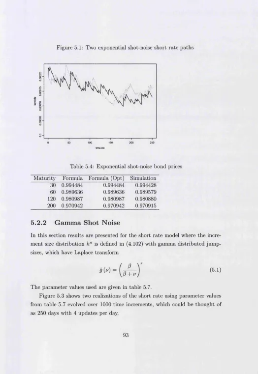
5.2.2 Gamma Shot N o ise ... 93

5.2.3 Double Gamma Short R a t e ...95

List of Tables

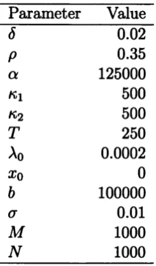
5.1 Parameter values u s e d ...91

5.2 Exponential shot-noise option prices... 92

5.3 Parameter v a lu e s ... 92

5.4 Exponential shot-noise bond p r i c e s ... 93

5.5 Exponential shot-noise option prices... 95

5.6 Simulated exponential shot-noise option p ric e s ... 96

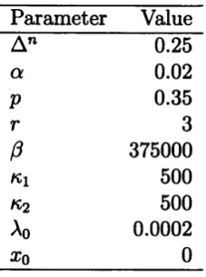
5.7 Parameter v a lu e s ... 97

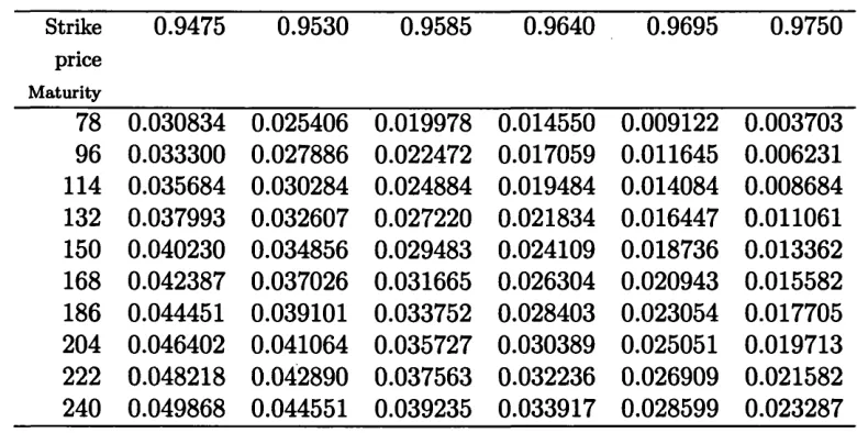
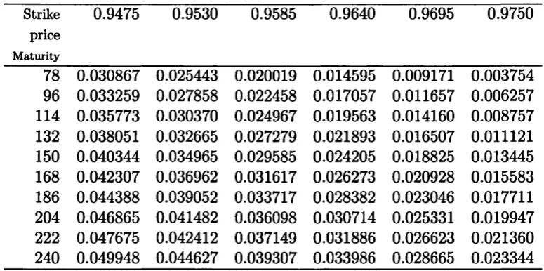
5.8 Gamma shot-noise bond prices...97

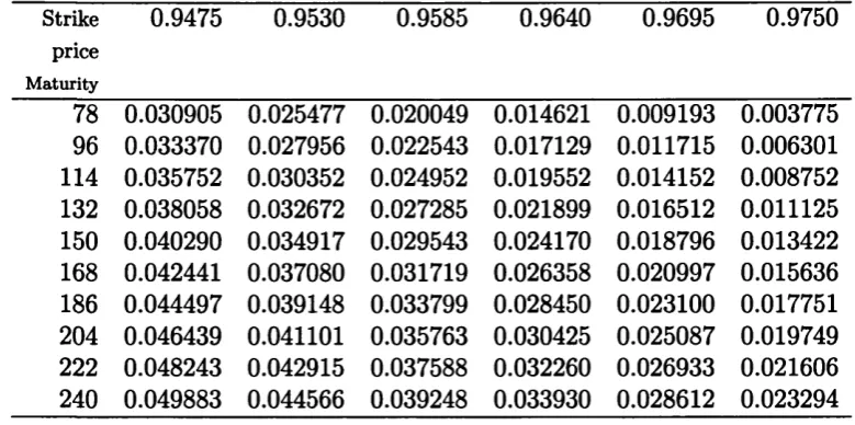
5.9 Gamma shot-noise option p ric e s ...99

5.10 Gamma shot-noise option p ric e s...99

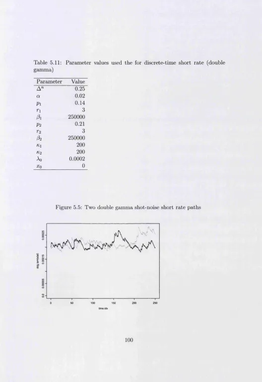
5.11 Parameter v a lu e s ... 100

5.12 Double Gamma jump bond p ric e s ...101

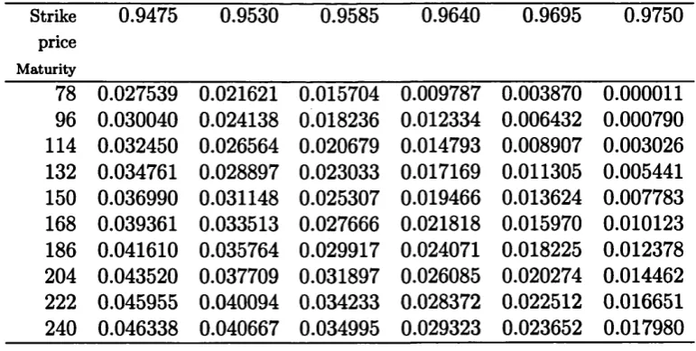
5.13 Double Gamma short-rate option prices... 102

List o f Figures

5.1 Two exponential shot-noise short rate realizatio n s... 93

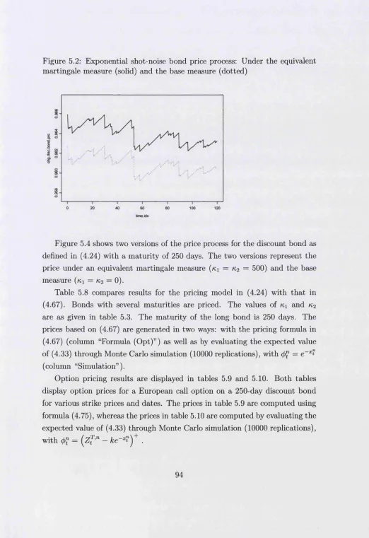
5.2 Exponential shot-noise bond price process ... 94

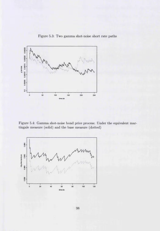
5.3 Two gamma shot-noise short rate re a liz a tio n s ... 98

5.4 Gamma shot-noise bond price process... 98

5.5 Two double gamma shot-noise short rate re a liz a tio n s... 100

Chapter 1

Introduction

1.1

M artingales and A rbitrage

Martingale theory has provided a suitable framework for pricing securities,

particularly contingent claims. A key element of this framework is the exclusion

of arbitrage opportunities, which started with the work on option pricing by Black and Scholes [6].

Harrison and Kreps [26] relate the concept of arbitrage to the valuation of contingent claims in a general setting for the discrete-time case using results

from martingale theory, while Harrison and Pliska [27] expand these results

to the continuous-time case. See Harrison and Pliska [27] and Baxter and Rennie [5] for specific derivations of the Black-Scholes option pricing formula

th at are based more explicitly on the relation between martingale theory and

the absence of arbitrage than that of Black and Scholes.

This section summarizes some results of the work mentioned above relevant

to this thesis. The notation used in Harrison and Pliska [27] will be adopted in what follows. We begin by calling into existence a probability space (fi, T , P)

and filtration {Pt\ 0 < t < T}, satisfying the usual conditions (see Harrison and Pliska [27] or Protter [35]). In a frictionless market with unrestricted borrowing

and short selling let the price processes (which are right continuous with left-

assumed to evolve from time 0 to time T. Security zero plays the role of a cash bond, the price of which, if it is absolutely continuous, may be written

f* \ ds

as eJo a where Xt is interpreted to be the instantaneous short rate at time

t. It will be convenient to normalize the price processes by dividing by the price of security zero. Thus the discounted price processes Z°, Z 1, . . . , Z K are obtained, where Z° is identical to 1 for 0 < t < T.

A trading strategy ip = {<pt : 0 < t < T } is defined to be a predictable vector process with components <p°, ip1, . . . , ipK. The vector process <p is pre­ dictable if its components (pl, i = 0 , . . . , K are measurable with respect to the a-algebra generated by the adapted processes with left-continuous paths. A

strategy (p defines a portfolio with value process V (ip) = X)£=o (p'S1. The gains process of portfolio (p is defined to be the stochastic integral G (ip) — f <pd,S = EiLo f <pldSl or Gt ((p) = Jo <pudSu. A strategy ip is said to be self-financing if

V (ip) = Vo (p) + G (ip), where Vo (ip) is the initial value (investment) of the portfolio.

The portfolio may also be viewed in terms of the discounted securities. The

discounted value process is defined as V* (ip) = 0ipxZ % = ipQ+Y$L i (f t^ t and the discounted gains process as G* (ip) = f ipdZ = I ip'dZ*. Harrison and Pliska [27] prove that <p is self-financing if and only if V* (ip) = V^* (<p)+G* (ip).

Next the existence is assumed of at least one measure P* which satisfies the following: 1) P* is equivalent to P and 2) the discounted price processes

Z1, . . . , Z K are P*-martingales. It will be necessary to determine the existence of P* in specific applications. If such a P* exists then for predictable ip1 the stochastic integrals / ipldZ% are local P*-martingales. Moreover, because the

Z x are positive, / ip'dZ1 are supermartingales under P*.

An arbitrage opportunity is defined to be a self-financing strategy ip such th at Vo (ip) = 0, Vo (ip) > 0 for 0 < t < T, but Vt (ip) > 0 with positive prob­ ability. There can be no arbitrage opportunities if an equivalent martingale

measure exists. This is because, as mentioned above, under any equivalent martingale measure P*, V* (ip) is known to be a positive supermartingale and thus must remain zero if it starts there. Under certain conditions the reverse

implication also holds true yielding the Fundamental Theorem of Asset Pric­

equivalent to absence of arbitrage. See, for example, Schachermayer [37] for

a proof of this theorem when time is finite discrete. Other treatments of the

theorem can be found in Harrison and Kreps [26], Harrison and Pliska [27] and

Delbaen and Schachermayer [15, 16].

A contingent claim is defined to be a positive, integrable random variable X

(by convention T = Tt, thus X is .Fr-measurable). Such a claim is attainable

if there exists a self-financing strategy such th at V f (<p) = (Sj.)-1 X , then

(p is called a replicating strategy and tt = Vq (ip) the price associated with

X . Traditionally the trick has been to limit the range of trading strategies

<p to predictable processes for which V* (tp) is a P*-martingale, in which case

7r = E* [Vf (ip)] = E* [(Sj.)-1 x j . Attainability is then defined with regards to this more limited set of strategies. A market is complete if all contingent

claims are attainable. If a market is complete then the equivalent martingale

measure is unique, see Harrison and Pliska [27].

The search for an equivalent martingale measure is thus justified in two

ways. Firstly, finding at least one equivalent martingale measure implies the

model does not allow arbitrage opportunities, providing an economic rationale to support the theory. Secondly, if the securities market is complete the mar­

tingale measure is unique and yields a unique price for any contingent claim. Completeness is a fairly specialist property, which even minor modifications

of a complete model may not possess. Examples are diffusion processes with

a stochastic volatility component and stochastic processes with jumps. This

thesis explores an incomplete model of the latter type. When the market is no longer complete not all contingent claims are attainable. The absence of

arbitrage is still implied by the existence of an equivalent martingale measure,

but as this measure is no longer necessarily unique, neither is the price of a

non-attainable contingent claim.

Since no replicating strategies exist for an non-attainable contingent claim,

one possible approach is to choose a strategy th at is as close as possible to a replicating strategy according to a some (subjective) criterion. Follmer

and Sondermann [22] drop the condition that a replicating strategy be self- financing. In their approach the strategy is certain to have a terminal value

out-flows during its lifetime. The strategy is chosen by minimizing a risk func­

tion, which is defined as the expected value at present of the square of the cash

flows to the strategy incurred over the remaining time to expiration. Follmer

and Sondermann [22] only consider the case where K = 1 and the discounted price process is already a martingale under the base measure. It turns out

th at the risk minimizing strategy is mean-self-financing, th at is the cost pro­

cess, defined to be the accumulated cash flows to the strategy, is a martingale.

Follmer and Schweizer [23] extend this result to the general case where the discounted price process is a semimartingale and the strategy is locally risk-

minimizing. Schweizer [39] provides an overview of the above as well as the

alternative approach, mean-variance hedging, where the replicating strategy

is required to be self-financing and where the expected value of the squared

difference between the value of the replicating portfolio at expiration and the

pay-off of the contingent claim is minimized.

1.2

Interest R ate M odels

The main topic of this thesis is the pricing of securities th at axe contingent on

interest rates. As with all securities, martingales and arbitrage play a key role in pricing those that depend on interest rates. An extensive literature is de­

voted to this topic, but the paper by Heath, Jarrow and Morton [28] is central.

In this paper the authors build on the work of Harrison and Pliska [27] to con­ struct a unifying theory for valuing contingent claims under a stochastic term

structure of interest rates. Their model, based on diffusion-type processes,

describes a complete market with a unique equivalent martingale measure and

unambiguous prices for contingent claims. The earlier companion papers by

Cox, Ingersoll and Ross [8, 9], also describe a term-structure theory based

on diffusion-type processes, but do not use the martingale theory-based ar­

gument of no-arbitrage to value securities. Instead, their approach is based

on economic equilibrium. Baxter and Rennie [5] provide an overview of the various term-structure models available in the literature th at are special cases

of the very general Heath-Jarrow-Morton (HJM) model.

gous to section 1.1, a probability space (17, T , P) and filtration { T t\ 0 < t < t}

describe the uncertainty in the economy and evolution of information, respec­

tively. Default-free discount (zero-coupon) bonds trade with various maturities

T € [0, t]. The price at time t of the T maturity bond is denoted by P (t, T). It

is required th at P ( T , T ) = 1, P ( t , T) > 0 for t € [0,T] and <9 log P (£, T) / d T

exists.

The instantaneous forward rate at time t for date T > t is then defined by

f { t , T ) = - d \ o g P ( t , T ) / d T for T E [0, r ] , t e [ 0 , T ]

This rate represents the forward price at time t of instantaneous risk-free bor­

rowing at a later time T. It follows that

P ( t , T) = exp

The short rate at time t is the instantaneous forward rate at time t for date t

and is given by

A* = / (£, t) for t e [0, t]

The value of a continuously compounding cash bond or deposit is then given by B t = efoXads, the same as security 0 from section 1.1 above. This se­ curity will have the special role of being a numeraire for other securities. Thus the discounted zero coupon bond price is Z (t, T) = B ^ l P (£, T). Under the assumption of no arbitrage an equivalent martingale measure P* exists th at allows a given interest rate contingent claim to be priced according to

B tE* F t ), where X is the pay-off at expiration. A direct consequence is th at the discount bond price is given by P (£, T) = B tE* •

In the HJM model the forward rate curve evolves over time according to a

(possibly multi dimensional) stochastic process. Though many popular interest

rate models are defined in terms of a short rate process, they can be written as

a forward rate model along the lines of HJM. The interest rate model examined

in this thesis is a short rate model. Instead of a diffusion-type process, however,

the short rate model is based on the discontinuous shot-noise process. Unlike

HJM, this model describes an incomplete market. The approach in this thesis

follows th at of Dassios [10], Dassios and Jang [11, 12] and Jang [31], where

the model has been explored extensively in an insurance mathematics context.

The shot noise process is introduced in the next chapter.

1.3

O verview

This dissertation is organized as follows: Chapter 2 presents an overview of

the shot-noise process. An important martingale is introduced which leads to

an expression for the joint Laplace transform of the interest rate and its time

integral. The martingale is also used to define an equivalent martingale mea­ sure based on the Esscher transform. These results will be used in subsequent

chapters to derive results for pricing interest rate contingent claims. Finally, a

short overview is given of the important affine jump-diffusion model, of which

the shot-noise process is a special case.

Chapter 3 develops some results in a continuous-time risk-neutral pricing

context. An interest rate model based on the shot-noise process is introduced. The price of a zero-coupon bond is derived by taking the expectation of the

discounted pay-off under an equivalent martingale measure. The derivation of this result relies on the Laplace transform from Chapter 2. A method is

presented to invert the Laplace transform when the jumps of the joint noise process are assumed to be exponentially distributed. This yields the joint

probability density function of the interest rate and its time integral, which is

used to compute the price of a call option on a bond, by taking the expectation of the pay-off under an equivalent martingale measure. The Laplace inversion

method used here is well-known in the telecommunications literature [1, 2]

as it is well suited for problems in queuing-theory, but we are unaware of its

application heretofore in the field of mathematical finance.

In Chapter 4 a discrete-time interest rate model is introduced, which has as

a special case a discrete-time version of the shot-noise process. This model is

more general, however, and allows for non-deterministic paths between jumps.

The discrete nature of this model makes it easier to price a non-attainable

security by tracking the value of a replicating portfolio th at is designed to

target security at expiration. The replicating strategy is derived by solving a

recursive optimization problem. Using this methodology, a general contingent

claim, which has zero-coupon bonds and European call and put options as

special cases, is priced by forming replicating portfolios of a longer-dated zero-

coupon bond and a cash account. The derived pricing formula is closed-form

up to an expectation operator. The expected value is evaluated using Laplace

inversion techniques in the context of a discount bond as well as a European

call and put option. The expectation result is closed-form in the case of the

bond while numerical Laplace inversion techniques are required for the options. These techniques lead to numerical evaluations that have not been before and

the option pricing result is central to this thesis. The equivalent martingale

measure implied by the mean-variance replicating bond price is examined and

an explicit representation for the Rado-Nikodym derivative is derived. This is

also a new result.

The model in chapter 4 is parameterized so that the length of the time- increments can be made arbitralily small. A limit argument then ties much

of the discrete-time theory developed in 4 in with the continuous-time model

presented in chapter 3. The framework developed for pricing bonds and Euro­ pean call and put options on bonds allows for a rich set of short rate processes

th at are discrete-time approximations to processes which can include multiple

sources of jumps and diffusion-type behavior between jumps. These results are another novel contribution of this thesis to the mathematical finance literature.

Chapter 2

Overview o f the Shot N oise

Process

2.1

Introduction

This chapter presents an overview of the shot-noise process. Much of the theory is based on piece-wise deterministic Markov processes introduced by Davis

[13, 14]. We give an overview of the generator and the extended generator of a Markov process. Next, the shot noise process is defined along with its

generator. An important martingale is introduced which leads to an expression for the joint Laplace transform of the shot noise process and its time integral.

The martingale is also used to define an equivalent martingale measure based

on the Esscher transform. These results are from Dassios [10], Jang [31] and

Dassios and Jang [11] and will be used in subsequent chapters to derive results

for pricing interest rate contingent claims.

Finally, a short overview is given of the important affine jump-diffusion

model, of which the shot noise process is a special case. This is based on

2.2

Strong G enerator

In this and the following section notation similar to that in Davis [14] will

be used and the reader is referred to this publication for further details. Let

(Ft) , (xt) , (Px, x € E)) be a Markov family on a state space E. The initial distribution is 6X, i.e. Px [xo = x] = 1, while the transition function p is related to the measure Px by

Px [xt

e

and satisfies the Chapman-Kolmogorov equation

p ( t + s , x , A ) =

f

JE

The expectation operator associated with the above Markov family is then

defined as

Ex [f (*<)] = / f ( y ) p (t, x, dy)

JE

If we let B (E ) denote the set of bounded measurable functions on E we may define an operator Pt : B (E) —> B (E) by

Ptf ( x ) = Ex {f {x t)} (2.1) Note th at Ptf (x) is again a function of x, the initial value of the process x t .

The Chapman-Kolmogorov equation is equivalent to the following semi-group

property of Pt for all s , t > 0,

PtPs = Pt+8

for any function / (x) in B (E), for which this limit exists. The strong generator can be regarded as a generalization of the derivative of Ex [f (x*)] with respect to t evaluated at 0. It can be proved (see Davis [14] or Oksendal [33]) th at

EX [/ (*«)] = / ( * ) + Ex [jf A f (xu) du (2.3)(2.3) for any stopping time t > 0. This is known as Dynkin’s formula. The set of functions for which the limit in (2.2) exists is called the domain of A and

denoted by D .

2.3

E xten d ed G enerator

Consider the Markov process x t from the previous section. Let D (A) denote the set of functions f in B (E) for which the following property holds: for every / G D (A) there exists a measurable function hf : E —» R (which may vary with / ) such th at the function t —►h f ( x t) is integrable Pz-a.s. and the process

is a martingale, where t > 0. We can then write A f (x) = hf (x) and call A

the extended generator of the process x t. We write

which is essentially the same as (2.3), Dynkin’s formula. It is often much (2.4)

Taking expectations on both sides gives us

E x [Cl\ = Ex [f (xt)] - Ex [f (x)] - Ex A f (xu) du = 0

As C{ is a martingale, Ex | c / | = Cq = 0 for any stopping time t > 0, and thus

of D (A) than of D ( a ) .

2.4

T he Shot N oise Process

The shot noise process consists of a series of random jumps occurring at poisson

times. In between jumps, process decays deterministically at an exponential

rate. The following definition is from Dassios and Jang [11]. At time t the process is represented as

At = Aoe- * 1 + J 2 V i e ~ i { t ~ Si)

all t «j<t

where:

Ao initial value of A

2/i size of jump i with 2/* > 0 and E (2/*) < 00

Si time at which jump i occurs, where s* < t < 00

S exponential decay

p the rate of jump arrival.

The jump-size distribution is denoted G (y). The aggregated process x t is defined as the time-integral of Af:

Xt = f Xads Jo

Following Jang [31] and Dassios and Jang [11], a slightly more general type

of shot noise process will be considered, where the parameters and jump-size

distribution depend on time:

(PDPs), a general class of non-diffusion stochastic processes, developed by

Davis [13, 14].

Using the fact that the triplet (xt, At, t) is jointly Markov, the notation in (2.1) can be adapted to suit the particular case of the shot noise process

Ptf (x, A, 0) = E [ f (art, At, t)\ (x0, A0,0) = (ar, A, 0)] (2.7) When conditioning on a starting point different from (x, A, 0), (2.7) implies

th at

P t f (xa, As, s) = E [ f (xt+a, At+8, t + s)\ (x„ Aa, s)] (2.8) Also, the generator of the generalized shot-noise process described above, act­ ing on a function / (x, A, t) is given by

A f (x, A, t) = ■— + A ^ - S (t) A ^ +

P (t) JjT + / (x, A 4- 2/, t) dG (y; t) - f (x, A, t)j (2.9) where the domain of the generator, D (A), is the set of functions / such th at for all i = 1,2,. . . ,

• / is absolutely continuous on R + x R + x [s*-!, s»), that is, between jumps.

• ^ [ | / ( ^ i5As<,s i) - / ( x ai,A8r ,s i)|] < o o

This follows from the results presented in Davis [13, 14] and is stated directly

in Jang [31].

The next result is from Jang [31] and can also be found in Dassios and

Jang [11].

P rop osition 2.4.1 (Theorem 2.1.11 by Jang) For constants k , v > 0 and the aggregated process x t associated with a generalized shot noise process Xt as

defined above, the function defined by

e~VXtexp f * e - W d r ^ A t ^ X

is a martingale where A (t) = JqS (s) ds and g is the Laplace transform of the jump-size distribution G.

Proposition 2.4.1 leads directly to the next useful result:

C o ro llary 2.4.2 The joint Laplace transform of Xt2 a n d x t2, given , is

e- "1**1 exp ( - / 1‘J e-A<r>ifr^At,) X

exp ( —f** p(s) |^l— f*2 e-A*rW;a^ j da) (2.11)

Proof: Because (2.10) is a martingale

E e~VXt2 exp ^fceA(t2)-^eA(t2) f*2 e - ^ d r j X t ^ Tt, x exp (/0t2p(a)[l-5(fceA<*>-i/eA(a> f* e- A<r>dr;a)]ds) =

e~VXt1 exp ^ - ^ f c e ^ ( t1) _ | / e A ( t 1 ) f*1 e-AWdr^Xt!^ X

exp (jjj1p(a)[l-g(keAM-veA<s> f* e-A(r>dr;«)]da)

Substituting v = V\ and k = z/2e_A^ + v\ Jq2 e~A^ d r into the above produces

the desired result in (2.11). Note that from (2.11) and the fact that \ t is a Markov process, it follows that

eUlXti E [e~UlXt2e ~ ^ Xt2\ j rtl] = E

Also note th at x t denotes a specific scalar-valued process in this section and is distinct from x t in the previous section where it denotes any (possibly vector­ valued) Markov process. In fact, (xt, Xt, t) in this section taken together as a single vector-valued Markov process is analogous to x t from the previous section. For the special case 5 (t) = 5, the martingale in (2.10) reduces to

e—Kr,e—(*e«-*(e«—1))A, ^ (2.12)

to

e - , z te-(*e«-*(e«<-l))At exp (p j^ [l-a(fce^-y(e*._1))]rf.) (2.13)

Assume the latter case, where no parameters depend on time. Let Xt describe the short-rate process. Then the value of a cash bond (or deposit) at time t

is eXt. The extended generator of (xt,Xt,t) acting on a function / (x, X,t) is given by

A f ( X,X,t) = g + A | - a | +

P [j^ + f ( x , X + y, t) dG (y) - f (x, A, t)j (2.14) a result found in Dassios [10] and a special case of (2.9).

2.5

T he Esscher Transform and E quivalent

M artingale M easures

The Esscher transform is a tool borrowed from actuarial science, as noted in

Gerber and Shiu [25], which has also proved useful in finance. The transform induces an equivalent martingale probability measure on certain stochastic

processes which can be useful in valuing derivative securities. Gerber and

Shiu [24, 25] apply Esscher transforms to option pricing for several types of stochastic processes. Biihlmann, Delbaen, Embrechts and Shiryaev [7] discuss

Esscher transforms as they relate to the no-arbitrage argument in mathemat­

ical finance. Jang [31] applies the Esscher transform method to the pricing of insurance derivatives.

Let P* denote a change of measure, equivalent to P. Then the expectation with respect to P* is defined as

E* P*

X T (2.15)

martingale Mt — E [ ^ | Pt\ as

E* Y Mt

Ms Ts (2.16)

The Esscher transform allows us to reverse-engineer P* by defining M t as follows: Let R (x, A, t) be a measurable function such that Mt = eR(Xt'Xt,t^ is a martingale. Then we will use Mt to define the Radon-Nikodym derivative as in (2.16). This Radon-Nikodym derivative is a special case of the Esscher transform. For any measurable function / the expectation of the random

variable f (xt, Xt,t) with respect to the newly defined probability measure is then given by

E- [ / ( * „ A * t) |* ] = [}[E [ e ’(:t M \ r s] ' J (2-17) The following result is due to Jang [31], where it is proved in the slightly

narrower context of the strong generator.

T h eo re m 2.5.1 Let x t andXt be as defined above. Let A denote their extended generator given by (2.14) and let A* denote the extended generator of (xt, At, t) under the new measure given by (2.17). Also, let R be a function as defined above and furthermore satisfy the same restrictions as f given below (2.9). Then A* acting on a function f (xt, At,t) is given by

A \ f ( x , X , t )

1 eR(xAt) !- a . e . (2.18) Proof: Let P denote the base measure with respect to which the process

(xt, At, t) is originally defined and let P* denote the change of measure implied by using eR(Xt,Xt^ to define the Radon-Nikodym derivative. Recall from the previous section th at A f ( x t,Xt ,t) is defined to be the process hf (xt, Af, t),

where h f (x, A, t) is a measurable function of (x, A, t), such th at the process

is a P-martingale. Similarly, for (2.18) to hold, we need the process

d f = /(* « . K t) - f (0, A„, 0) - 1 X eR(J ^ U u (2.19) to be a P*-martingale. As C*^ is adapted to F t, for t > s we have

E>

[c;!

-I.

(2.20)

We will examine the last term more closely:

rt A [ / (xu, Au, u)

)Au jti)

* tp*

\ ^

(Xui

^R{x\i j At* )U)

du

j

M

F a \ =

rt ^ f A [ / (xa, As, s) eR{-Xa >a)]

J,

-F A du = du =

r>{

gi2(ls,Aa,s) dr (2.21)

In the first and second step above we made use of the Fubini theorem and

Markov property of (xt, At) t), respectively. The operator Pt* is defined analo­ gous to (2.7) and (2.8). Using (2.17) yields

Pf f (x8, ^81 s) — E [ f {,Xt+8i ^ ^)| (^sj ^)] exp (R (.xt+s, Xt+a, t + s)) f (xt+8, ^t+si t s')

E tJ e x p (P (x a, Aa,s)) Pt [/ (x3, A3, s) exp (P (a:3, A3, s))]

exp (R (x8, \ S,s))

(x s, A 3, s)

Substituting (2.22) into (2.21) results in

J f Pr { ^ iR (*«■ A»> *»} dT

exp (R (xa, As, s))

Pt_a [/ (xs, Aa, s) exp (R (x8, Aa, s))] _ / (xa, Aa, s) exp (R (xa, Aa, s)) __ exp (R (xa, A5, s) ) e x p ( R ( x a, \ a,s))

p t - 3 If (x a, As, s)] - / (xa, Aa, s) (2.23) The RHS of the first equality in (2.23) follows from (2.5). In order to use (2.5)

the function / ( x , A,£)exp(R(x, A, t)) must he in the domain of A, which it does by the restrictions imposed on R in the hypothesis. Noting th at

E* [ f (xt, Xu t)| T a\ = Pt*_a [f(x„ As, s)]

then shows th at the last term in (2.20) cancels out the first two. We conclude th at C*^ is a martingale and thus that the generator of (xt, At, t) is character­ ized by (2.18).

We now turn to a specific form of eR^XuXut\ namely a slightly rewritten version of the martingale given in (2.13):

_ g—niSxtg— («i+K2e5t)AtgP/0*[l—fl(«i+K2e5a)]ds

Here and n2 are constants such that «i > 0 and k2 > —Kie~6t* and it is

assumed that the process evolves up to time t*(see Dassios [10] for details). Thus R (x, A, t) has the following form:

R (x, A, t) = — K\Sx — + n2eSt^ A + P

J

The Radon-Nykodim derivative process may then be defined as

In order to find A* f (x, A, t) we will need A { / (x, A, t) Define

ip(x, A, t) = / (x, A, t) eR(x,x,t)

From (2.14) we know that

A<p(x,X ,t) = & + \ ? g - 6 X j £ +

P <p(x,A + y, t) dG (y) - <p(x, A, *)j (2.25)

Furthermore, it is easily verified that

d t ~ \ d t + J d t )

^ = e«(xA<) ( dJ - + f f ) OX \ o x ox J & P _ eR(x,X,t) ( W + f 9 R \

d x ~ \ d x ± J d x )

dR = -SK 2e6tX + p [l - g (aci + K2e6t)\

OR(x, A, t)

and

where

and

dx —KiS

Additionally,

<p(x,X + y ,t) = f (x, A + y ,t) e- ( 't*+«e<*)>'efl(x'A't) Substituting the above equations into (2.25) yields

A<p(x, A, t) =

eR(xX‘)p \ J / (x, A + y, t) (y ) - f (x, A,«)] (2.26) And thus

where

P f f ( x , \ + y, t ) e ' ^ + ^ d G (y) -JE+

p f ( x ,\ ,t ) g ( K i + K2e6t>)

= % + x % ~ s x % + p t {t) L f { x , x + y ' t] d G ' { y ' t]

(2.27)

P* (t ) = pg («i + K2est) (2.28) and

rfr* r„-rt e - {K1+K2e“)vdG(y)

d G (y , t) - g ( K i + K 2 E s t )~ (2'29)

This result is due to Jang [31] (Theorem 3.2.5) where it is noted th at (2.27)

is a special case of (2.9) and thus, under the new equivalent measure P*, Xt

follows a generalized shot noise process with time-dependent parameter p* (t )

and time-dependent jump-size distribution function G* (y; t).

We will now obtain an expression for the joint conditional Laplace trans­

form (LT) of (xt, Xu t) under the equivalent martingale measure P*. This result can be obtained in two ways: Firstly, by using the generator A* in (2.27). The second way is by using the Laplace transform under the base measure P , given

in (2.11).

We start by using the result in (2.27) combined with (2.12). Since

is a P*-martingale we have

E |exp^-i/*t2-(fccit2_^^eit2-i^At2+J’ p*(a)[l-ff*(fce5a-^(e5*-l);«)]da^ |^rt1 j —

e~UXtl exp (-(fce**i-£(e**i-l))Atl) exp (f*1 p*(s)[l-p* (***--£ (e*8-l);a)]da) Take

and

which implies

1/1 = v

i/2 = ke5t2 — ^ (e^ 2 — l)

i/2e~6t2 + ( l — e~5t2>) = k

and thus

kelt' - - (eil1 - l ) = + y ( l - e~s^ - ^ )

This leads to

E* =

e-v\xtxeXp ^ _ ^ e-i(t2-*i)+f^(i-e-i(t2-*i)))At1) X

exp ( - / tt2p*(s)[l-fl*(y2e-^t2--)+^ (i_ e -tf(t2-«));s)]ds) =

e”*'1**1 exp X

exp ^-p/[p(Ki+K2e{8)-p(»^e-6(t2-®)+f^^i_e-i(t2- fl))+/ci+/C2ei*)]da^ (2.31)

The second method allows us to prove the result in (2.31) without the trans­

formed generator. Using the joint Laplace transform of x t2 and Xt2, given Xtl, in (2.11) leads to

e-(n+KiS)xHe-(n+ n+ Ka^ ) x a exp (p J^ -^ m + w * * )]* )

E ( e -* l{*'se-('tl+',2e<‘2N exp (p £ s[i-i(« + « ^* )]* )| ^ j . )

%' t \

exp ^-p J^2 Jl-p^(iA2+«i+K2etft2)e-«(t2-«)+lil^UiI(i-e-«(*2-*))^jdaj

e-/ci5a:tie -(«i+«2etfti)At1 exp ^ Jjj1 [i-^Kx+Kae*-)]*)

e-{v\+K\S)xtx exp ^_^l^e-i(t2-ti)+K2e«i)-|-i^(i_c-5(t2-ti))+/c1)At1) X exp ^p j'0t2[l-p(«i+/C2ei*)]tfa^ X

exp ^-p/ t*a Jl-5^(wa+Ki+K2eft2)e-^t2-*)+^JSl^(l-e-a(*2-»))JJ<l8^

e-mSxHe-(Ki+K2eSti)Xtl exp ^ j t t [1_3(#Cl+#taC*#)]<kJ

e~UlXtl exp (-(^2e-5(t2-*x)+i^(l-e-^t2-*i)))At1) X

exp (pf£[g(!£ - ( !£-V2)e-6(t-2- e')+Ki+K2eSs)-g(Ki+K2eSB)]ds>j

which is the same result as (2.31), yielded by using the generator.

2.6

Affine Jum p-D iffusion M odels

The shot noise process described above is a special (and simple) case of a more

general class of processes called affine jump-diffusion (AJD) processes. AJD

models nevertheless have sufficient structure to yield closed- or nearly closed- form expressions for securities prices and many models of the term structure

are special cases. For an introduction to AJD term-structure models, see

Duffie and Kan [18]. Duffie, Pan and Singleton [19] develop an option pricing

methodology within the AJD framework. Duffie et. al. [17] provide a rigorous

definition and characterization of regular affine processes.

Following Duffie, Pan and Singleton [19], but modifying the notation to

conform to the previous section, the AJD model is defined as follows: Let a

differential equation

d(t — p, (£t) dt + (j (£*) dBt + dJt (2.32) where B is an (J^)-standard Brownian motion in Rn; p : D —> R n, o : D —> R nxn, and J is a pure jump process whose jumps have a fixed probability

distribution G on R n and arrive with intensity {p (Ct) : t >0}, for some p :

D —> [0, oo). The generator of the process in (2.32) acting on a function / (£) is then given by

A f { Q = + ^ rtr(C M C )1’ +

dC .dC

P ( 0 [ [f(C + y ) - f (C)] dG (y) (2.33) An affine structure is imposed on the functions /i, aaT and p. Moreover, the short rate is also assumed to be affine in its dependence on the state variable £. The affine structure has made the model in (2.32) analytically tractable

compared to its general form.

Comparing (2.33) to (2.14) it is immediately clear th at for n = 1 and trivially affine transformations p, (x) = — Sx, a (x ) = 0 and p (x ) = p, the SDE in (2.32) defines a shot noise process.

The framework for the AJD models allows for an extension of the shot-

noise process, described in section 2.4, by adding a Brownian perturbation.

This process will be referred to as a diffusion shot noise process and is defined by the SDE

dXf; — —5 \tdt ■+■ crdBt dJ% (2.34) Let its aggregated process x be defined by

xt = f

Jo

func-tion / (x, A, t) is given by

d f . , d f t s d f . I # 2/ 2 A /( *, A ,t ) = — + A5 i - * A g j + 2^ +

P [jf + / (x, A + j/, t) dG (y) - / (i, A, t) (2.36) W ith (2.36) it is possible to extend the result in (2.13).

T h e o re m 2.6.1 Let A and x be as defined in (2.34) and (2.35), respectively, evolving up to a fixed time t*. Also, let and«2 be constants such that «i > 0

and k>2 > —Kie~St*. Then the process given by

g KiSxtg («1+/S2e )At eXp J*^i_^Kl+K2e6a^ds_ la2 (2.37)

is a martingale.

Proof: Following Dassios [10], define

wt = 6xt + A* and

Zt = Xte6t

We will try a function of the form

/* (to, z, t) = e~Klwe~K2Zh(t) = e- ^ + » e- < ^ ‘h ^ or

/ (x, A, t) = /* (fa + A, \ e st, t) = e- KlSxe - ( '1+K2eSt)xh (t) (2.38) Substituting (2.38) into (2.36) yields

A f (x t A, t) =

e- M ( t ) p ^ ^ + K2e« ) _ x] Setting this to zero yields

t i (t) = h (t) p ( l - g (ki + «2e5t) ) - («i + Ac2e<5t) 2J (2.39) Solving for h (t) results in

h (t) = K exp jp /04[l—<7(/ci+K2e*a)]ds—§a2 ^(/ei+^e**)2* } (2.40) where K is an arbitrary constant. This completes the proof.

Theorem 2.6.1 leads directly to a generalization of the result in 2.11.

C o ro lla ry 2.6.2 The joint Laplace transform of Xt2 and x t2, given Atl is

E [ e - ^ ^ e - ^ l ^ ] =

exp | — P jf ( l — 5 (vi 1~e~S^ 2~a) dsj x

exp|^cr2jf (vi1- e~y?~") +U2e~s(t2- g)^ dsj (2.41) Proof: Because (2.37) is a martingale,

E ^ y e '*iix*2“(Ki+K2e 2)*t2 expj^J, ^p(l-p(/ci+/c2e5a))-^ (« i+ K2etf5)2j<isj

J

=

e KiSxtl e ( K l+ K 2 e )^* 1 exp J o*1 ( l - g ( « 1+iC2e5 a) ) d « - J < T 2 ^ ^ ( j s x + ^ e * ® ) 2 * ]

(2.42)

Dividing both sides of (2.42) by

exp f*2 r p ( l —<7(«i+K2e*a) ) —^-(/ci+Ktte*41) Ida•

n L J

and substituting the values «i = ^ and «2 = (^2 — ^ ) e yields the desired

Chapter 3

A Continuous-Tim e Interest

R ate M odel

3.1

Introduction

This chapter introduces an interest rate model based on the shot-noise process

described in chapter 2. The price of a zero-coupon bond is derived by taking

the expectation of the discounted pay-off under an equivalent martingale mea­ sure. The derivation of this result relies on the Laplace transform results from

Chapter 2.

Weeks’ method to invert Laplace transforms is introduced and applied in the context of a shot-noise process with exponentially distributed jumps. This

yields the joint probability density function of the interest rate and its time integral, which is used to compute the price of a call option on a bond, by taking

the expectation of the pay-off under an equivalent martingale measure. This

equivalent martingale measure is often interpreted as a risk-neutral measure

and this approach to option pricing will be referred to as risk-neutral valuation.

Though Weeks’ method is well-known in the telecommunications literature,

as it is well suited for problems in queuing-theory, its current application to

3.2

D efinition o f th e M odel

We will use the shot noise process At with parameters p and S and jump size distribution G (y) (all independent of time), as defined in section 2.4, to model the instantaneous short rate. Also, let x t denote the aggregate process /o Aads. The shot noise process is a suitable model model for an interest rate because it does not assume negative values as long as the domain of the jump-

size probability density g is R +. Clearly, a model that produces occasional negative short rates is unrealistic because interest rates are rarely below zero. People are usually not paid to borrow money. That said, there are examples

of interest rate models where the short rate is allowed to go negative. The Ho

and Lee model is an example (see Baxter and Rennie [5] for an overview).

The generator of the Markov process (xt, At, t) acting on a function / (x, A, t)

is given by (2.14). The value of a continuously compounding cash bond or de­

posit is now given by B t = eXt. Let P ( t,T ) denote the price at time t of a zero-coupon or discount bond maturing at time T and let Z (t, T ) denote the corresponding discounted bond price process B ^ P (t,T ). We will use P to denote the original measure with respect to which ( \ t,x t,t) is defined and P*

to denote an equivalent martingale measure, suitably chosen with the aid of

an Esscher transform as described in section 2.5.

As discussed in sections 1.1 and 1.2, a bond maturing at time T may be viewed as a contingent claim with payoff 1 at time T and thus may be priced within a risk-neutral framework as P (£, T) = B tE* 1 , where E* is the expectation with respect to P*, an equivalent martingale measure. As it turns

out, the equivalent martingale measure is not unique, even when it is defined using the Esscher transform Mt, defined in (2.24). Recall th at according to

(2.27), under this new measure, the process is a generalized shot-noise process,

the parameters of which are given right below (2.27). We will use (2.12) to find

an expression for the discounted bond price process Z (t , T) = E*

In fact,

is a P*-martingale and thus we have

E * ^ e -„ xT e - ( k e St-%(e*T- l ) ) \ T e fo p*(s)[l-g*(kes>-^(e6>-l);s)]ds^:F^ =

e~VXte~ (fee6<” * (eSt-0)x* efo p* (•) [w* (ke*a~ i(e69 ~1) ;*)]* or

E * ^ e - UXTe - ( keSt~!s(eST-1))XT\ j rt^ =

e - v x t e - ( k e St- % ( e St- l ) ) \ t e - p * (s)[ l-g * (ke Sa- % ( e 6a- l ) ; a ) ] d s

We will choose v —1 and k = ^ ( l — e~ST^j. This yields

E * (e~ XT\ f t) =

Recall from (2.27), (2.28) and (2.29) that the generalized shot-noise process in question is defined by

P* (t) = pg («i + n2est) and

yv' ’ g(Ki + W “ ) It is easily established th at

» • ( { ; . ) - / .

y VS y J R+ ^ ' Jr+ g(K !+ K 2eSt)

g ( i + K i + ^ e St)

g («1 + n2est)

/ X \ r £ ( l ( 1 - e 5(T a)) + «1 + /c2etfs) (Kl + K2e6‘) 1 - l M i '

>-v 1 9 («i + «2eds)

P[0 («i + «2e6s) - § 0 ( l - e_<J(T_s)) + «i + /c2e*s) j

We finally obtain the desired expression for the discounted bond price process

Z ( t ,T ) = E ’ (e “IT|5 i ) =

e- n e- J ( j- e - J(T- ‘))A,e>>/tT[S(isi+K2e<'+ j(l-e -,(T-*)))-s(it1+/C2es')]<i>

(3.1)

Z (t,T ) is a P*-martingale, because

E ' [Z (t, T )\T ,\ = E * {E * [e~XT\ E t] \ E ,} = E ‘ [e~XT\ E , ] = Z ( s , T )

We will not worry about how K\ and k2 should be determined but assume they have been chosen suitably in some sense.

If K\ and «2 are zero, i.e. assuming no change of measure, the price process for a discount bond maturing at time T is

P ( t,T ) = e- K1- ‘- i(T- ‘))**e'/.T[KH‘- ‘- s<I' - )) J - 1!*

As was pointed out in section 2.6, the interest rate model defined in this

section is a special case of the affine jump-diffusion process presented in Duffie,

Pan and Singleton [19]. It is not surprising that the change of measure they propose is equivalent to the Esscher transform used above when their model is

limited to the special case of the shot noise process. In fact, since the shot noise

process becomes a generalized shot noise process with deterministic, but time-

dependent parameters under the change of measure, the affine structure of the

model is preserved, just as in the more general case of the AJD model. This

allows the machinery developed for affine processes to be used for derivatives

pricing and it is easily verified th at the AJD model leads to the same bond

price as in (3.1). Beyond preserving the affine structure of the model, the issue

The remainder of this chapter is in line with this philosophy and assumes that

a suitable change of measure has already been decided on. Chapter 4 will

address the choice of equivalent martingale measure in detail, albeit indirectly.

3.3

Inverse Laplace Transform

3.3.1 In trod u ction

The Fundamental Theorem of Asset Pricing justifies pricing a contingent claim

by computing the expected value of the pay-off at expiration under an equiv­

alent martingale measure. The pricing formula for a discount bond in (3.1) is

an example of this approach, which also illustrates the key role th at Laplace

transforms play, especially when the discounted pay-off at expiration can be

written as an exponential function of an affine combination of Xt and Ar, where T is the expiration date.

Duffie, Pan and Singleton [19] pursue a similar approach for pricing claims by using a type of extended Fourier transform. Specifically, using the notation

in section 2.6, the extended transform of given the information available at time t, is

E exp R ( ( a,s)ds^J (uq + Ui - (T)e u<T Tt (3.2) where the short rate R is an affine function of £r, possibly time dependent, and Vo, v\ and u may be complex-valued. This extended transform differs from the (conditional) characteristic function (Fourier transform) because the discounting at rate R (ft, t) and the term v0 + v\ • Ct- Though a closed-form expression for (3.2) will automatically produce a closed-form expression for the

price of a discount bond, pricing more complicated claims, such as options, is

more involved. As an example, Duffie, Pan and Singleton [19] consider the

price at time 0 of an option that pays off (ed'^T — cj at time T, for given

price of the call option at time 0 is then

P = Gd - d( - log c) - cG0,-d ( - log c)

The function Ga,b (z) is given by (3.2) for the complex coefficient vector u =

a + izb, with Vo — 1 and V\ = 0. Because of the affine structure of the model, a closed-form expression exists for the Fourier transform of the function Ga,b (•) defined by

roo

Ga,t(z)= e ' * v d G a , „ ( y )

J —OO

The closed-form solution is

Ga,b(z) = eam + m < °

where a and (3 solve known, complex-valued ordinary differential equations with boundary conditions at T determined by z. In some cases these ODEs have explicit solutions, in others they need to be solved numerically. The

function Ga,b (•) can then be be obtained by inverting the Fourier transform

Qa,b (*)• This example in the beginning of Duffie, Pan and Singleton [19] is fairly typical of their approach toward pricing various types of options.

The approach pursued here in the context of the shot-noise process is some­

what different. In (2.31) an expression was presented for the joint conditional

Laplace transform of x t and At, given and Xtl for t\ < t, under the equivalent martingale measure P*. The simple nature of the shot-noise process, when jump-sizes are assumed to be exponentially distributed, allows for an explicit

evaluation of the Laplace transform in (2.31). The inverse Laplace transform is

equivalent to the joint conditional probability distribution of x t and Xt- Given a few regularity conditions, with the inverse transform the conditional expected

value of many types of functions of Xt and At can be computed, allowing for the evaluation of a general set of contingent claims. The remainder of this sec­ tion will focus on the implementation of Weeks’ method of Laplace transform

inversion. Though implementing this method requires numerical integration,

it produces a closed-form expression of the inverse Laplace transform, which

At- In the next section the inverse Laplace transform will be used to compute

the price of a European call option by taking the conditional expectation of

the pay-off at expiration under the equivalent martingale measure P*.

3.3.2

Laplace Transform

Abusing our notation slightly, we will denote the conditional joint probability

density of x t and \ t, given T tx, by II (xt, At), ignoring any reference to J^ .T h e next theorem presents the Laplace transform of II for the specific case when

the jump sizes follow an exponential distribution.

T h eo re m 3.3.1 Let A and x be as defined in section 2.4, where S and p are time-invariant and the jump-size distribution is exponential, that is

g(y) = ae~ay (3.3)

and its Laplace transform is

(3.4)

Then the joint L T of x t2 and Xt2, given Atl under the measure P*, as given in (2.31), takes on the specific form

H (uu u2) = E , { e~nXt* e~nXt? \ f tl} =

e~n x’i exp exp x

a + Ki

+

(l -

^

a + «i +

p a

f a + Ki + K2e 6tl A \ a -I- Ki + K2e St2)

Proof: Recall from (2.31) that

exP (~ /.‘2 (^+(*-2- ; « ) ] < < » )

Also, recall from (2.28) and (2.29) that

P* W = P9(«1 + «2e*) and

e- ( K1+K*p-St)ydG (y) 9 (ki + K2e5t)

Using (3.4) yields

P* W = _{a + Ki}pa _{+ K2eSt}

g* (y; t) = (a + Kl + K2est) e-(«+ «iW *)v and

Thus

and

9* to * ) = a + /ci + <St

9* =

a + «i + ^

a+Ki+«2Ca*

a+Ki+^+^K2+(v2-^-)e 5t2)e'<5t

pa

a+Ki+Q+(K2+(v2-^)e St2^e5t

From (2.31) it is clear th at we need to evaluate

£ p* (a) [l - y* (^ .+(^-^)e-*<*J- ) i.)] ds =

}

f-Ju Iti [a+Ki+K2ea* I a + « i+ ^ + (/C 2 + (i/2 - i^ )e 6t2)ea* ds (3.6)

Both terms in the integral on the RHS of (3.6) are of the form • These

integrals may be evaluated as follows:

L

*2 ds _ 1 re**2 du ti A + Be68 S Jesti (A + Bu) u

1 M _

<5 Je6ti [Au

B

We have

f eSt2 du 1 , ,e«t2 S {t>2 — ti)

L ~Au = ~A [ gulcSl1 = A (3-8)

and

/'

J e (

,St2 _du

1 , ( A + Be6t2\

= B l0 g t

fest1 A + B u

Substituting (3.8) and (3.9) into (3.7) yields

A + Be6ti) (3-9)

I rest 2

5 JeSt l

B

Au A (A + Bu) d “ = S i \-5 (*2 “ J l ) " log ( ^ f $ r ) ] ( 3 1 0 )

Applying (3.10) to the two terms on the RHS of (3.6) yields

r t2

J t i OL

pads

pa

and

pads

[ * f e - f l) - l o g ( s ± a ± 2 g ) ] (3.11)

rt2

hi a

Ki

pa

S t 2

S t i

S + Ki +

S (t2 - ti) - log ( ---«+K1+Ky“ 2 + v ' V tt+fCi+^e'

(3.12)

Thus combining (3.6), (3.11) and (3.12) yields

exp <

-{ - / ?

pet pot_________________ I i I __

a+Ki+K2et* a + fs 1 + ^ + ( K 2 + ( * ^ - ^ ) e - 6 t 2 ) e ^ J J

/ g+K1+>C2e^tl+t/2e~g^2~tl^ + ^ ( 1- e~^^2~tl^)^ ^(<*+«l)+*'l

y g+«l+»s2e^t2+,/2 /

pot

e x p ( ^ - < o ( ^ - ^ ) ) ( g ^ ) “+“‘ (3.13)

The desired result follows from substituting (3.13) into (2.31).

3.3.3

W eeks’ M eth od

For the purpose of pricing a European call option we will need to invert (3.5)

w.r.t. i/2- It will become clear at the end of section 3.4 why (3.5) does not

need to be inverted w.r.t. i/\. In a nutshell, the option pricing formula derived will turn out to have the form of a Laplace transform wrt x t2. Though this inversion problem is not known to be analytically tractable, techniques exist

to approximate II (z/i, v2) with a linear combination of functions (of 1/2) whose inverse Laplace transforms axe known.

The inversion technique applied here is based on Laguerre polynomials and

known as Weeks’ method [40]. Though this method was one of the first suc­

cessful implementations, the idea of using Laguerre functions to invert Laplace transforms goes as far back as Widder [41]. He proved that, under certain

regularity conditions, the inverse transform may be represented as an infinite weighted sum of Laguerre functions. Many transform inversion methods based

on th at of Weeks have been proposed since. An example is th at presented in

the companion papers by Abate et al. [1, 2], which describe a method for the univariate and multivariate cases, respectively. The paper by Kano et al.

[32] provides a description of Weeks’ method and an extension to the case of

matrix functions.

The description of Weeks’ method by Kano et al. [32] is presented next,

adapted to the present context. Weeks’ method returns an analytical formula

for the inverse transform function. It assumes that a function II (x) can be represented as an expansion in terms of Laguerre polynomials L n (x)

00

The Laguerre polynomials Ln(x) form an orthogonal basis in L2 (R) and are commonly used to approximate functions. The two scaling parameters a and

b need to be chosen so th at b > 0 and a > ao, where oq is the abscissa

of convergence. If the infinite Laguerre expansion converges uniformly then

II (x) may be approximated for numerical purposes by

N

n

n=0

where N is chosen so th at the error of the approximation is below the desired tolerance.

The principal challenge is to compute the coefficients Cn, which is described next. Given a Laplace transform II (i/), its inverse is defined as a contour integral in the complex plane

where i = y[—\ and T is the Bromwhich contour T (i/) = <t + iy, with a > obj

y € R. Then

roo ^

II (rc) = —— / e*yxn (a + iy) dy (3.16)

Z 7 T J —oo

Equating (3.14) and (3.16) yields

° ° 1 roo ^

Y Cne'^Ln (2bx) = — / etyxU (a + iy) dy (3.17) 7 1 = 0 2 ? r J ~ ° °

The weighted Laguerre functions have the Fourier representation

l 3 ' 1 8 )

e - b x

Substituting (3.18) into (3.17) and interchanging sum and integral, which is

valid if (3.14) converges uniformly, leads to

Next, a Mobius transformation is applied to map v to a new complex variable

w

Using v = a + iy leads to and the inverse is

v — a — b w =

---v — <7 + b i y - b iy + b ib (w + 1 )

w — 1

w =

y =

CnWn = (iy + 6) ft (a + iy) = ft (cr - 6 ^ 4 ) 1 - i u V w - l j

The coefficients c„ may be computed using Cauchy’s integral formula by inte­

grating along the unit circle w = etd

Cn = —

f

T " ( < 7

-27r y-7r 1 — etd \ e10 — 1J

The resulting inversion formula is then

n w -

E ( i

■»)

<*•>

For numerical purposes, the coefficients Cn need to be evaluated via numerical integration. Using the midpoint rule leads to the approximation

Cnr*j

e j m _ 2b ^ 2M _{m = —M} 1 - ei0m+1/2

^ ( eWm+l/2 1 \

(32°)

where 6m = m = — M , . . . , M — 1 and n = 0 , . . . , iV.

Kano et al. [32] also provide error bounds for the approximation due to

readily available in e.g. [4].

The Laguerre polynomials Ln (x) can be defined via the generating function (1 - t y 1 e~—< = £ L„ (*) tn (3.21)

n = 0

Laguerre polynomials satisfy the well-known triple recursion relation

L„ (x) = 2n ~ 1 ~ X£ n_t (x) - — 2 ( i) (3.22)

n n

which may be proved with (3.21) or by using their orthogonality property [4].

The recurrence relation in (3.22) can be useful for computing the values of the

Laguerre polynomials to evaluate the approximation in (3.15). It is possible,

however, th at the Laguerre polynomials become large as their order increases,

which can lead to a prohibitive loss in precision. In this case Kano et al. [32] recommend evaluating the sum in (3.15) by using the backward Clenshaw

algorithm as described in [34]. In the applications in chapter 5 there is no

apparent need for using the backward Clenshaw algorithm and it has not been

implemented here.

We will need to evaluate integrals of the form

I n ( x ,v ) = [ Xe - * L n (y)dy (3.23)

Jo

The generating function (3.21) may be used to develop a recursion th at is

useful for computing (3.23). Evaluating the integral of the left-hand side of (3.21) yields

i rx vt 1 — e~xve~x *=*

(1 — t)

f

l - e - ^ ( l - t ) E ” 0Ln ( s ) t w (1 — t) v + 1

Equating this to the same integral of the right-hand side of (3.21) yields

0° oo

1 - e~z" (1 - 1) £ L n (I ) t" = ( ( l - t ) u + t ) ' £ tn/„ Or, v)

or

oo oo

1 _ e— £ L„ (*) t" + «— £ L„ (*) <"+> =

n =0 n=0

oo oo

V tnIn (x, v) + (1 - v) tn+1In (x, v)

n =0 n=0

Equating powers of t leads to

r / . . A l - e ~ ~ L o ( x )

Iq (X, 1/j —

V

and

e

xv

if

In (x, v) = (Ln_ 1(x) - Ln ( x ) )---— In-1 (x, v)

When x —► oo the integral in (3.23) becomes the Laplace transform of

Ln (y). It is well-known, see e.g. [1], th at the Laplace transform of Ln (y) is 1 » M = iHSo7" ") = ('/^ + i ) (3-24)

Since n(i/i,j/2) is assumed to be known from the outset, it can be used to assess the accuracy of the app