The economics of income tax evasion

Incom e Tax Evasion

A thesis presented

by

R alph-C . Bayer

to

The Department of Economics

in partial fulfilment of the requirements for the degree of

Doctor of Philosophy

in the subject of

Economics

London School of Economics and Political Science

All rights reserved

INFORMATION TO ALL USERS

The quality of this reproduction is dependent upon the quality of the copy submitted.

In the unlikely event that the author did not send a complete manuscript and there are missing pages, these will be noted. Also, if material had to be removed,

a note will indicate the deletion.

Dissertation Publishing

UMI U615605

Published by ProQuest LLC 2014. Copyright in the Dissertation held by the Author. Microform Edition © ProQuest LLC.

All rights reserved. This work is protected against unauthorized copying under Title 17, United States Code.

ProQuest LLC

789 East Eisenhower Parkway P.O. Box 1346

This thesis consists of three extended essays on the evasion of income tax. The main purpose of this thesis is to refine the existing tax evasion models in a way th at makes it possible to explain empirically established stylized facts th a t could not be explained before.

In the first part we use a standard neoclassical framework in order to analyse the impact of risk preferences on evasion behaviour. We argue th a t expected value maximization with some fixed and variable costs incurred during the evasion process (moral cost, cost of coverage action etc.) is an appropriate framework to explain the stylised fact th a t higher tax rates and a higher income lead to more tax evasion. This resolves one of the puzzles concerning tax evasion th at was unsolved so far.

1 In trod u ction ... 10

2 Incom e tax evasion, opportunities, and evasion costs ... 15

2.1 Introduction ... 16

2.2 The m o d e l... 18

2.2.1 Opportunities and evasion c o s ts ... 18

2.2.2 Attitudes towards r i s k ... 21

2.2.3 Tax system ... 23

2.2.4 Detection, penalties and expected payoff... 24

2.2.5 Optimal underreporting... 26

2.3 Comparative s ta t ic s ... 27

2.3.1 Changes in the tax s y ste m ... 28

2.3.2 Changes in the individual param eters... 30

2.3.3 Changes in the enforcement param eters...32

2.3.4 Honest taxpayers, evaders and ghosts... 33

2.4 The general case: income and policy effects... 36

2.4.1 Tax system, penalty scheme, and evasion c o st... 37

2.4.2 Optimal reported income ...43

2.4.3 Changes in gross incom e...46

2.4.4 Policy effects...47

2.5 Simulating the German tax sy stem ...50

3 A contest w ith th e ta x m a n ... 60

3.1 Introduction ... 61

3.2 Timing and basic assu m p tio n s...65

3.2.1 T im ing... 65

3.2.2 The basic assum ptions... 66

3.2.3 The pay-offs and some n o ta tio n ...70

3.3 The case of perfect and complete inform ation... 73

3.3.1 Solving by backward in d u ctio n ...74

3.3.2 E q uilib ria... 76

3.3.3 Comparative statics ... 80

3.4 The case of complete, but imperfect inform ation...83

3.4.1 E q u ilib ria... 84

3.5 Signaling with hidden a ctio n ... 91

3.5.1 Equilibria for different parameter settings... 92

3.6 Extensions for the signaling settin g ...103

3.6.1 Externally enforced incentive com patibility... 103

3.6.2 Non dichotomous probability distributions...107 •

3.6.3 Privately known moral c o s t ... 113

3.7 Conclusion...117

3.A Proofs of some propositions...120

4.2.2 Crooks and good citizens ...132

4.2.3 Pay-offs... 133

4.2.4 Simplifying assu m p tio n s... 135

4.3 Optimal efforts... 140

4.4 Auditing with g h o s ts ...142

4.4.1 Ghosts with simultaneous a u d itin g ...143

4.4.2 Ghosts with sequential a u d itin g ... 148

4.4.3 The sequential auditing p a th ... 156

4.4.4 A numerical e x a m p le ...163

4.5 Equilibria in mixed stra te g ie s... 165

4.5.1 Simultaneous a u d itin g ... 166

4.5.2 Mixing with sequential a u d itin g ... 170

4.5.3 Mixing in a numerical exam ple... 172

4.6 Self-selection of moonlighters...173

4.7 Conclusion...177

4. A Some proofs of propositions in the main text ...178

5 Lessons for ta x authorities and g o v ern m en ts...182

5.1 A uthorities...182

5.2 Governments... 184

Figure 2.1 The 1983 tax system and its approximation ... 51

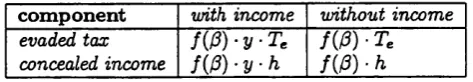
Figure 2.2 Simulated concealed income...53

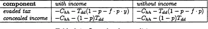
Figure 2.3 Legal, simulated, and empirical tax r a t e s ...54

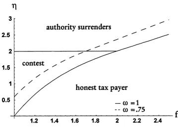
Figure 3.1 Parameter configurations for perfect information equilibria...81

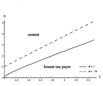
Figure 3.2 Parameter configurations for imperfect information equilibria... 87

Figure 3.3 Parameter configurations for pure evasion and hybrid eq u ilib ria 97 Figure 3.4 Evasion probability and waste pecentage for different tax r a t e s 100 Figure 3.5 Waste percentage for different earning probabilities...102

Table 2.1 Potentially fair penalty schemes...40

Table 2.2 Fair penalty factors... 41

Table 2.3 Global fair gamble conditions for fair penalties... 45

Table 2.4 Second order conditions... 45

Table 2.5 Effects of policy changes... 48

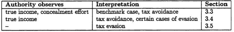
Table 3.1 Different informational s e ttin g s ...73

Table 4.1 Expected ghost and deviation pay o ff...163

C hapter 1

Introduction

This dissertation consists of three self-contained essays on income tax evasion. They basically form the chapters in this thesis. However, there is a common pur­ pose. The aim of the work presented here is to give positive explanations for some phenomena linked to tax evasion. There is an old puzzle in the tax evasion litera­ ture. Why are people evading more taxes when tax rates are raised, while evading less if the gross income decreases? These empirical observations seem intuitive on the one hand, but were hard to explain with models. The aim to find a satisfying explanation runs through this thesis like a thread.

would be the forces th at drive the results. Our approach to tackle the problem is the following. The observation that tax reports are repeated yearly suggests th at the scope of risk involved in tax evasion is limited; so rather some costs associated with cheating than risk aversion might be the factor that limits tax evasion. We introduce risk neutral taxpayers th at have to bear some fixed and variable costs if they evade taxes. Certainly, the risk neutrality assumption is just a very rough approximation for the real risk preferences. The fixed evasion costs come from personal attitudes and values. Moral constraints, the fear of stigmatization, peer group pressure are in­ cluded there. The variable evasion costs - depending on the scope of evasion - are expenses to create evasion opportunities, to cover the evasion, and forgone profits or income from restructuring economic activity. W ith such a setup we are able to show th a t higher tax rates and higher gross income lead individually to more tax evasion. This holds for a very wide range of tax and sanction systems observed in reality. Non-regressive tax systems and penalty schemes th a t take into account the scope of evasion and/or the economic ability (income) produce the observed relations between tax rates, income and evasion.

between tax inspector and evader, which is often observed in reality. We use this signaling game with two sided moral hazard to check whether the result from chap­ ter two (higher taxes and higher income lead to more tax evasion) still holds in this richer framework. Fortunately it does. Apart from this specific question, the pre­ sented model is of further, purely theoretical interest. As far as we know a model with this structure does not exist in the literature. There are many real world applica­ tions, where such a model could be used. Insurance fraud, benefit fraud, loan fraud, and sales of goods like antiques and paintings, where it is costly to prove authenticity, are some examples.

An additional feature of the model worth mentioning is th a t the authority cannot commit to an audit effort before observing the tax declaration. Together with the ability to choose tax and fine schemes the possibility to commit - as widely assumed in the literature - leads to models, where the revelation principle holds. This means th at there in equilibrium unrealistically no evasion takes place. For this reason we believe th at generally the non commitment assumption is more realistic.

For similar reasons we do not allow the authority to have control over tax and fine schemes. We think th at it is too narrow a view to search for an optimal tax structure just with respect to tax evasion. We confine the normative part of the paper to the analysis of the effects the tax rate has on resources wastefully invested in the contest. As intuition suggests, it turns out th a t higher tax rates do not only lead to more evasion, but to more wastefully invested resources as well.

th at taxpayers may have earnings from different sources, we show that it usually is optimal to audit these sources sequentially until some suspicion th at evasion took place arises. In the case of proven or suspected evasion during previous checks a full-scale audit of the remaining sources with a high effort will follow. Our result stems from a setting where taxpayers have different moral costs of evasion. These costs are private information. By auditing sequentially the tax inspector can update his beliefs about the type of taxpayer he faces. This leads to the possibility to better tailor the detection effort with the information from previous audits in hand.

be optimal for a taxpayer to split his activities if possible. He may prefer to work in both the official sector where all income is declared honestly, and in the black market economy where all income is evaded.

C hapter 2

Incom e ta x evasion, evasion

op portu n ities, and evasion costs

2.1

Introduction

The still widely used neoclassical framework for the analysis of income tax evasion was set out within the seminal papers of Allingham & Sandmo [1972] and Yitzhaki [1974]. One of the most important questions in these early papers were: How do tax­ payers (and evaders) react to changes in the tax rate, and do people evade more when they get richer? Certainly, the intuitive answers are: Higher tax rates lead to more evasion and richer taxpayers will ceteribus paribus evade more. And in fact, econo­ metric studies suggest th a t in this case intuition is a reliable guide (see e.g. Clotfelter [1983], Dubin, Graetz &; Wilde [1987], or Feinstein [1991] for influential econometric studies, Andreoni, Erard &; Feinstein [1998] and Bayer &; Reichl [1997] contain more recent surveys). Unfortunately, the early models couldn’t simultaneously reproduce the empirically observed relations in a convincing manner. Furthermore, the compar­ ative static results were not very robust against small changes in the tax and penalty schemes. In a setting where the penalty depends on the evaded tax [Yitzhaki 1974] and risk-averse taxpayers maximize expected utility the two effects even unambigu­ ously point in different directions. When tax evasion increases w ith the gross income it decreases with the tax rate or vice versa.

ble explanations of the puzzle, while the latter lacked the robustness against small arbitrary changes of functional forms.1

The second generation of tax evasion models - initiated by Reinganum Wilde [1985] - came from game and contract theory. These papers (see e.g. Border & Sobel [1987], Mookherjee & Png [1989], Mookherjee h Png [1990], or Chander & Wilde [1998]) rather searched for an optimal, incentive compatible, environment by optimizing tax, penalty and audit schemes, than to try to solve the puzzle described above. Economic psychologists - mainly in experiments - found a variety of influence factors for tax evasion. But the resulting frameworks were mainly descriptive and did not have too much predictive power for expected behavioural reactions on changes in the environment (see Webley, Robben, Elffers & Hessing [1991] for a good overview).

This chapter tries to provide a solution of the tax evasion puzzle by stepping back to the early models, where we slightly change some assumptions. We assume risk-neutral instead of risk-averse taxpayers and argue th at this might be a viable approximation for the risk preferences in the case of tax evasion. This assumption is justified by experimental evidence and psychological theories. In some models dealing with optimal taxation and tax evasion [Cremer &; Gahvari 1994], or with the black market economy [Cowell & Gordon 1995], this assumption has been used to keep the models tractable. Furthermore, we introduce evasion costs, such as the fixed moral cost of doing something illegal or the variable costs for concealing income and creating opportunities to evade.2

1 For a recent review of the relevant theoretical and empirical literature see Slemrod &: Yitzhaki

[2002],

In the following section the assumptions are justified and an “example” , which has the generality level of the early models, is set up. The comparative statics in section 2.3 show th a t we can reproduce the empirically observed effects. Section 2.4 extends this result to a wide range of tax systems, penalty schemes, and evasion cost functions. The main conditions for our results to hold are a non-regressive tax system and what we call a “fair” penalty scheme. In section 2.5 we show in a simulation th a t our model is able to reproduce empirical real world data. The simulation results for the German 1983 tariff are compared to estimates from individual income data reported by Lang, NOhrbass h Stahl [1997]. We conclude with some final remarks.

2.2

T he m odel

2.2.1

O pportunities and evasion costs

Different taxpayers have different opportunities to evade taxes. These different op­ portunities may stem from different sources of income. For example employees have few possibilities to evade their working income, since their taxes in many countries are directly collected and delivered to the tax authorities by the employer.3 Oppor­ tunities to evade have to be created. Collusion with the employer and working in the shadow economy are examples for creating such opportunities. On the other hand, self-employed taxpayers have some more means of evading taxes. They can simply not report issued bills or make too high deductions by handing in bills paid for pri­ vate purposes. These different opportunities also apply for other sources of income. We can think of gains from the capital markets as well. In Germany, for example, taxes on interest payments have to be collected and delivered by the banks in be­ half of their customers. It is not too easy to get around this legal evasion obstacle. But, there are cases where collusion between the banks and the taxpayers took place. This opportunity had to be created. By contrast, speculative gains from trading with shaxes are easy to hide.4

This story tells us two things. Taxpayers have different opportunities to evade, and since opportunities often have to be created or at least information about oppor­ tunities has to be gathered, underreporting is costly. Obviously, the opportunities to evade a person has are closely related to the potential evasion costs it has to bear.

3 This is e.g. the case in Germany and Switzerland.

The more opportunities a taxpayer has the easier it is for him to evade, and the lower are the evasion costs.

If we now consider a rational tax evader with an income y stemming from different sources, which is the first part of income he will underreport? Obviously, th e income from the source with the lowest evasion costs. Additionally, he will use the cheapest means of underreporting first. To conceal further income he might have to use costlier means and/or sources. In the German example for capital gains, a person with income from the capital market may first underreport his gains from share trading, which is related to low evasion costs, than bring some money abroad to create the opportunity to underreport interest payments, and than try to establish collusion with the bank, which is very costly indeed.

Thus, the additional costs for further evasion are positively related to the share of income already evaded. Furthermore, these costs decline with the individual op­ portunities to evade. To avoid the technical problem to deal with a discontinuous cost function we use a continuous cost function as an approximation.5 If we consider the relations being linear at the margin, the marginal costs of evading can be written as:

where h / y is the share of income not reported and 6 denotes the individual evasion opportunities. The total evasion costs depend on the unreported income h and can

be found by integration. This yields:6

c (ft) = { * +0& ; /

h

h >J0

(1)

The integration constant k can be interpreted as the initial fixed costs of evading; i.e. the cost for acquisition of information about opportunities to evade and the often claimed moral costs to do something illegal. Furthermore, they can be seen as the cost of the first monetary unit evaded. This fixed cost might be individually different as evasion opportunities are. Our notion of fixed evasion costs is related to the approach in Myles k Naylor [1996]. There an honest taxpayer enjoys some utility from conforming with other honest taxpayers. A motivation why there may be a utility loss simply caused by the act of evasion was first provided by Gordon [1989].

The quite arbitrary looking formulation of evasion costs is less crucial for the results to be derived later than one might suspect. The properties we need are Ch > 0, Chh > 0, Co < 0 and Cyh < 0, where subscripts denote partial derivatives.7

The explicit formulation is used for expositional reasons.

2.2.2

A ttitu d es towards risk

The crucial assumptions driving the results in the early tax evasion models are those about the risk preferences of the taxpayers. On the first sight, it seems very reason­ able to assume risk-averse actors, and consequently to use von Neumann-Morgenstern

6 We restrict the unreported income to be non-negative. In reality overreporting som etim es happens and is caused by mistakes or insufficient information. Since we concentrate on planed behaviour, these cases are not relevant in our setting.

expected utility functions. But the empirical evidence about risk preferences is some­ w hat mixed.8 Decision-making under risk is very sensitive against small changes in the environment. Hence, to use the same model structure for portfolio decisions with risky assets and tax evasion does not necessarily mean th a t it is sensible to use the same risk preferences, as well.9 In our opinion, it is possible to resolve many decision anomalies in the context of tax evasion, which are widely discussed in the economic psychology literature, by assuming - as an approximation - risk neutral taxpayers.

The specification of risk preferences according to the Prospect Theory proves a good working hypothesis [Kahneman h Tversky 1979]. Psychologically, changes in the environment th at lead to a reduction in (economic) freedom (e.g. higher tax rates) are very likely to lead to the so called reactance phenomenon (Brehm [1966] and Brehm h Brehm [1981]) if we consider the situation of the taxpayer’s reporting decision. Reactance - in this context - means th at people use an available instrument (here: tax evasion) to win back their freedom.10 This is the basis for the assumption of the risk loving taxpayer in situations where he wants to avoid a sure loss - as predicted by prospect theory. Beyond the reference point, where the prospect is a possible gain, it is reasonable to stick to risk aversion as an assumption, since the taxpayer sees the situation as a usual gamble - again, as prospect theory predicts.11

8 For a survey see Camerer [1995] or Camerer [1998]. An older, but more rigorous treatment is found in Machina [1987]..

9 For obvious deficiencies of expected utility theory see the stunning calibration exercise in Rabin

[2000].

10 There are several conditions determining whether reactance occurs and what reduction instru­ ments are used. The very interesting discussion about the consequences for situations where the Prospect Theory can be applied has still to be led.

B ut ju st to incorporate such preferences into a usual framework of tax evasion is not viable and needs further assumptions. First of all, the individual reference point has to be determined and, secondly, we have to decide the extent of risk aversion and risk love for the different net-income levels.

The assumptions about relative and absolute risk aversion (using von Neuman- Morgenstem utility functions) were crucial for the predictions of the early tax evasion models. We claim th a t in the tax evasion game - because of the game being played repeatedly and with high stakes - people are approximately risk neutral. For the case of losses and high stakes experimental evidence shows th at people are in fact approximately risk neutral [Kachelmeier h Shehata 1992]. Furthermore, the fact that the game is played repeatedly leads to the reasoning th a t the variance of the average period payoff (over all periods) is much smaller than the variance of an actual period payoff. This means th a t the uncertainty in the repeated game is much smaller than in the one shot game. This should reduce risk aversion. Evidence for this claimed effect was also found in the mentioned experiments of Kachelmeier and Shehata where gains or losses were added to or taken from virtual accounts.

In using risk neutrality as an assumption we have a fairly good approximation for preferences in risky games with high stakes, regardless whether they are consid­ ered as possible gains or possibly avoidable losses. In the case of tax evasion this assumption might be a better approximation than the traditional von Neumann- Morgenstern approach. In addition, we do not run into the problem of finding a reference point if we wanted to use the preferences proposed by the Prospect The­

ory. This makes our further analysis comparatively simple, and reproduces - as we will show - empirically observed behavioural reactions of taxpayers to changes in the environment.

2.2.3

Tax system

We use a progressive tax system to cope with reality On the other hand, to keep things simple, we assume in this example th at the tax rate is linearly dependent on the reported income. Furthermore, to ensure th at the decision function of the taxpayers is continuous and differentiable, we assume th at already for the first unit of income tax has to be paid and that the maximal tax rate is reached at the highest income in the population.12 Then (true) tax liability T for a certain income y is given by T(y) = t(y)y, with t(y) = Ty + a, where r represents the marginal rise of the tax rate with respect to income, which is a measure for the progression of the system. The q is a constant part of the tax rate. Variations of a can be used to change the tax rate for all incomes by the same amount. We get:

T(y) = r y 2 + ay. (2)

Certainly, to obtain the tax liability with unreported income, the true gross income y has to be replaced by the declared income d = y — hwhere h denotes the concealed income.

The assumed linear dependency of the marginal tax rate on the declared income is not crucial for our analysis. The main results hold, as long the tax system is not regressive.

2.2.4

D etection , penalties and exp ected payoff

As in the basic models of tax evasion we assume a fixed probability p of being audited. This can be interpreted as the given strategy of the tax authority being to audit a certain amount of taxpayers randomly. We assume further th a t an audit reveals the true income with certainty. If an audit detects underreporting the tax cheat will have to pay his true tax liability and an additional penalty. Here, we assume th at the penalty is a linear function of the amount of taxes the taxpayer tried to evade, which is T(y) — T( y — h) = h(a — hr + 2yr). Thus, denoting the penalty parameter by / , the payoff after an audit D(h) is given by

D(h) = y - T(y) - f[T(y) - T( y - h)} - C{h). (3)

We chose this specification of the penalty scheme, since this is the same as Yitzhaki [1974] used to find th at for a proportional tax system ( r = 0 in our setting) the relation between tax evasion and tax rate definitely has another sign than the relation between tax evasion and gross income.13 The main results hold as well for other specifications.14

On the other hand, if a tax cheat gets away with his underreporting his payoff G(h) will be his true income minus the tax payments associated with his reported

income and the evasion cost. This is expressed by the following equation:

G(h) = y - T { y - h ) - C ( h ) . (4)

13 There, for a decreasing (increasing) absolute risk aversion the relationship between tax rate and evasion is negative (positive), that between gross income and evasion is positive (negative).

Since .we assume th a t there is no reward for overreporting of income we can restrict h to values bigger or equal to 0 in both cases.15 A rational risk-neutral taxpayer

maximizes his expected ex post income by choosing an optimal level of non-reported income. The expected ex post income E( h) is the sum of the with their probabilities weighted pay-offs for the two states of the world; i.e. being audited or not:

E(h) = pD(h) + (I - p)G{h) (5)

2.2.5

O ptim al underreporting

Denoting the declared income (y — h) by d, the first-order condition for this maxi­ mization problem is given by:

dE(h) _, dT(d) &T(d) , dC(h) n

- d r - {1 - p ) - d r - p f - d r + - d T = 0 - (6)

Examining the first-order condition part by part we see th a t the first (positive) term is the expected marginal gain for a further monetary unit of unreported income, while the following (negative) terms are the expected marginal penalty for detected evasion and the marginal evasion cost of a further unit of unreported income.

We can find combinations of the auditing parameters / and p th at ensure th a t everyone reports truthfully. The condition deterring tax evasion is p + p f > 1. If this condition holds the marginal gain (net of evasion costs) of not reporting a unit of income is always negative. The gamble against the tax authority is an unfair one and no risk-neutral taxpayer will evade. Since in reality the parameters are such th at people evade taxes, we will not look at such cases. Bernasconi [1998] reports

p + p f = .054 for the US and similar values for other countries. So we restrict our parameters in a way th at the following inequality holds:16

p + p f < 1.

As easily can be checked, the second derivative is negative and the second order condition for a maximum is fulfilled if we impose this restriction:17

* E { h ) p m

a

c(fc)

- j u ? ~ = ( p + p f - iJ - g g s a s r < 0

-Plugging the values for our specification into the first-order condition (equation

6) and solving for h yields, an interior solution assumed, a closed form solution for

the optimal amount of concealed income fi*, which is:18

h. (1 - p - p f ) (2r y + a)

2t(1 — p —

1/

For an interior solution the tax gamble has to be fair and the fixed evasion costs k

have to be sufficiently small. In the following section we will assume this to be the case. For a further analysis see section 2.3.4.

2.3

Com parative statics

The standard models of tax evasion with taxpayers being risk-averse and having risk preferences, th a t are not affected by changes in parameters, are not capable of simul­ taneously explaining the empirically observed positive relations between unreported

16 For other specifications this ’’more than a fair gamble” condition is slightly more complicated. E.g. in the Allingham /Sandm o setting for fines we would get ps < 2 y r ( l — p).

17 This is the case since we assumed an indirectly progressive tax system (T " > 0) and increasing marginal evasion costs (C" > 0).

income and tax rates and between true and non-reported income. 19 So it is useful

to have a look on the relationships our model predicts. In this and the next two sections we will restrict ourselves to parameter settings with interior solutions. The conditions for corner solutions are examined in section 2.3.4.

2.3.1

Changes in th e ta x system

In the case of tax rate variations there are two different sub cases of interest. W hat happens,

1. if the tax rate rises due to a ceteribus paribus increase in the progression r,

2. if the tax rate rises for everyone by the same amount (increase in a)?

The marginal changes in non-reported income in equilibrium is given by implicit differentiation of the first-order condition. For case one, where the marginal tax rate rises, while the income independent component of the tax rate stays the same, the change in optimal underreporting is given by:20

dh

d r h=h- Ehh 1

/(

)

We already know that the second derivative of the expected ex-post income with respect to the unreported income is negative. Thus the sign of equation 8 is given

19 For the early basic models see Allingham & Sandmo [1972] and Yitzhaki [1974], who assume constant tax rates, Christiansen [1980] for progressive tax system s, and Clotfelter [1983] who estim ates the effects of changing tax rates with TCMP data.

by the sign of the numerator. It is obvious that for an interior solution (0 < h* < y ) ceteribus paribus the influence of the marginal tax rate on the unreported income is positive. This result holds for all non-regressive tax systems since the conditions for the positive sign are T y T > 0, T y y > 0 and Cfih > 0- The first condition can be interpreted as the fact that a ceteribus paribus rise in the progression, holding the tax rate for the poorest taxpayer constant, leads to a higher marginal tax rate. The second condition assures th at the tax system is not regressive; the third th a t the marginal evasion costs are rising with unreported income.

The second case, where the tax rate rises for everybody by the same amount, is represented in our model by a rise in a. Again, implicit differentiation of the first-order condition leads to the equilibrium change of the unreported income:

— = 1 - p - p f Q

da fc=h. l/(y9 ) + 2 r(l - p - p f)

We see th at the influence of an increased constant part of the tax rate on unreported income is positive as well.21 To see how tax evasion is influenced by changes in the

tax rate we have to examine the relation between evaded tax (denoted by F) and unreported income (h). This relationship is purely technical, and is determined by the tax system as the difference between the true tax burden and the tax burden with cheating:

F(h) = T(y) - T (y - h) = h(a - r h + 2ry) (9)

To find the change in the amount of tax evaded if one of the tax rate parameters rises, we have to examine the sign of the derivatives of F (h) in equilibrium with respect to the interesting parameters.

d F (h * ,a,-) dh* 0 d h * , . . . _

9 a “ a ~da + + "ga > (1Q)

dF (h*,r;-) dh* dh*

■3; • = + h * )(y -h ') > 0 (1 1)

We see th at both derivatives are positive. Considering the assumed inner solution for h* we can state th a t raising the tax parameters leads to more income unreported and through th at channel to more taxes evaded. If the taxpayer reported no income before, he will report no income after the change of the tax rate again. The relations shown above lead to the following Proposition.

P r o p o s itio n 2.3.1 In our example an increase in the tax rate, interpreted as an increase in r or in a, leads to

1. more income underreported,

2. to more tax evasion if an interior solution is realized before the tax rate change,

2.3.2

Changes in th e individual param eters

In our model, two individual characteristics, the gross income y and the evasion opportunity 6, are exogenously given parameters. Let us now consider the changes of the taxpayers’ behaviour due to exogenous changes in these parameters. It is quite obvious th a t a greater opportunity for evasion - exogenously determined by sources of income, knowledge of evasion possibilities, etc. - should lead to higher tax evasion. And indeed, a higher 9 induces more non-reported income, and ceteribus paribus more tax evasion. This is shown by the following equation:

dh

39 h=h- Eh$ E hh 6 + 20 ( l - p - p f ) / yh * > 0 (12)

As intuition and real world data suggest, the non-reported income should in­ crease with the gross income. The following implicit derivative shows that this is in fact true for our example, since the right hand side is positive, whenever an interior solution is achieved (1 — p — p f > 0):

dh dy

_ E ky h '/ ( y26) + 2 t(1 - p - p f ) „ . . B kh ! /( » * ) + 2 r( l - P - p f ) ~ V

This rather trivial result is quite important. Combining this result with the result of proposition 2.3.1 we get the empirically observed result that both relations - tax rate and income to evasion - point in the same positive direction. The existing theoretical literature could not unambiguously reproduce these empirical findings 22 A further

result we get is th at a taxpayer th at reported at least a certain amount of income (h* < y) will at least report a fraction of his additional income. This is true since the

implicit derivative in equation 13 is smaller than one in th at case. Using equations 12 and 13 we can state the following proposition.

P ro p o s itio n 2.3.2 Ceteribus paribus in our example,

1. a taxpayer will evade more (less) taxes the higher (lower) his evasion opportunity

is.

2. An interior solution assumed, rising income leads to more tax evasion, and

3. an additional unit o f income is reported at least partly, if the taxpayer reported some income before.

2.3.3

Changes in th e enforcem ent param eters

The most obvious results we get for the comparative statics of changes in the enforce­ ment parameters, i.e. the exogenously given auditing probability and the penalty scheme. As in the classic tax evasion models a higher audit probability p leads to lower underreporting. The same is true for higher penalties which is indicated by a higher penalty parameter / . Applying the same procedure as above to determine the sign of equilibrium changes in the non-reported income due to a variation of the enforcement parameters we get:

dh dp dh d f

h=h'

h=h-E hp _ (1 + f ) { a + 2r(y - h*) Ehh 1/{yO) + 2t (1- p - p f ) Ehf _ p(a + 2r ( y - h*)

Ehh ~ 1/(y6) + 2t (1 - p - p f )

< 0 and

< 0

The two equations above show th at audit probability and fines are both ap­ propriate instruments to lower underreporting, since both implicit derivatives are negative.23 As easily can be checked, the effect on the taxes evaded points in the

same direction.24 This is the standard finding in the tax evasion literature. More in­

teresting than this rather trivial statement is the question, which instrument is the more effective in reducing the amount of unreported income. To make the effects on underreporting comparable we derive the elasticities th at show the percentage of re­ duced underreported income as consequence of a percentage rise in the enforcement parameter. The two elasticities are:

Tlh',p

Vh-j

p dh h* dp f dh h* d f

h =h ‘

h =h ‘

{p + p f ) { a + 2r{ y - h*) h*

[

/

p f ( a + 2T(y - h*) h* [l / W + 2 r (l - p - pf)]

(16)

(17)

We immediately find th at the absolute value of the audit probability elasticity

7]h. p is higher than th at of the penalty parameter Ph%f- This means th a t - as empirical

evidence suggests - raising the audit probability is more effective than imposing more severe penalties.25 However, the desirability of using the instruments depends heavily

on the associated costs.

23 That is true for an interior solution (y > h > 0), which implies a gamble with positive expected value (1 — p — p s > 0). Note, that we assumed an interior solution to exist.

24 This is due to the implicit derivatives of th* having the same sign as equations 14 and 15.

P r o p o s itio n 2.3.3 Raising the audit probability and imposing higher fines are means of achieving lower underreporting, but audit probabilities are more effective

than fines.

2.3.4

H onest taxpayers, evaders and ghosts

Since we assumed th at there is an initial fixed cost k. of behaving as a cheat, for some taxpayers - in expected terms - it will not be profitable to evade taxes, even if the game is a gamble th at is better than fair. The taxpayer will compare the expected payoff she yields if she decides to bear the initial fixed evasion costs and chooses the optimal amount of underreporting with the certain payoff she yields if she does not evade. She will evade if and only if E(h*) > y — T(y). Dividing the net expected value in a gross component E{h*), which depends on the non-reported income, and in the fixed cost k we get the following condition for evasion E(h*) — k > y — T(y).

Solving for k we obtain the minimum fixed evasion cost to force an individual taxpayer to report truthfully:

k, = E (h m) - ( y - T(y)) (18)

To study the change of the behaviour of formerly honest taxpayers due to changes in personal or tax system parameters, we have to examine the change of this minimum fixed cost necessary to prevent cheating. If the reaction of ki is positive

and a continuous distribution of k exists, which assigns positive frequencies to the whole support of the distribution [0, /c^] with Kh > then at least one formerly

Since the fixed cost is an additive constant within the net expected payoff function, the implicit derivative of the net payoff with respect to the interesting parameters is equal to th a t of the gross payoff; i.e. dE(h*)/d(-) = dE(h*)/d(-). This gives the following equation that decides the change in /q for an individual taxpayer:

dK, dE(h>) d [ y - T ( y ) }

fl(-) a(-) d(-) u s ;

We immediately see th a t for changes in the parameters th a t have no influence on the net income after reporting truthfully; i.e. p, / and 0; we get the same sign

for our change in the minimum fixed evasion cost th a t deters from evasion as for the comparative static analysis above. In conclusion we can say - as intuition suggests - th a t lower audit probabilities and fines, as well as greater opportunities to evade, lead to more formerly honest taxpayers becoming tax cheats.

In the case of a higher tax rate we have to calculate d t y / d r and dKi/da. Both derivatives are positive:26

^ = (1 — p —p /) (2y — h')h* > 0 (2 0)

^ = ( 1 - p - p f W > 0 (21)

Thus, rising tax rates - from an increase either in the income-dependent (r) or the independent (a) component - induce formerly honest taxpayers to underreport their income.

The question whether a rise in personal income promotes honest taxpayers to become evaders depends on the sign of the following derivative:

^ = ft* (2( l - p - P/ ) + ^ ) > 0 (2 2)

The effect of a rise in gross income on a marginally honest taxpayer is positive as well. Summing up our findings about formerly honest taxpayers’ reactions to changes in the model parameters (from equations 2 0 to 2 2) gives us the following proposition.

P ro p o s itio n 2.3.4 Under the assumption that the fixed evasion cost distribution provides positive frequencies for all k € [0, R] such that there always exists at least one taxpayer that is indifferent between reporting his entire income or not reporting

h* we can say that there is at least one formerly honest taxpayer that starts cheating

1. if the tax rate ( r and/or a), the income (y), or the evasion opportunity (9)

increases, and

2. if the audit probability (p), or the fine rate ( f ) decreases.

Another interesting question concerns the condition under which a taxpayer prefers to declare no income at all and becomes what in the literature is called a “ghost” ? 7 To find the necessary (and for small k sufficient) condition for a taxpayer to prefer to be a ghost, we take equation 7, which determines the optimal non-reported income h* and set h* equal to y. Solving for 9 and recalling th a t h* increases with 9,

leads to the following handy inequality:

0 > - n_{a ( l}— "---(23)_{- p - p f )}

P ro p o s itio n 2.3.5 For sufficiently large opportunities for evasion, a high income independent part o f the tax rate, and for sufficiently low audit probabilities and fines

an individual taxpayer will become a “ghost” who reports no income at all.

2.4

T he general case: incom e and policy effects

We have already argued th at our findings about the taxpayers’ reactions on changes in parameters are quite general. In this section we show the necessary conditions for our main results to hold. For this purpose, we set up a general framework and formulate requirements for the functions th at ensure th at a taxpayer ceteribus paribus reacts with more tax evasion to higher taxes and to a higher personal gross income. More generally, we introduce a policy parameter 0 th a t the government can influence. This gives us the possibility of analysing the reactions of the taxpayer to certain policies.

2.4.1

Tax system , p en alty schem e, and evasion cost

Tax system

The tax system assigns a tax liability to every (declared or true) income. W ith­ out loss of generality we can specify the tax systems in terms of parameters:

T{y,(3) = t[y,0\y = [r(y,0) - z(y,0)]y (24) The tax system T(j/, j3) is assumed to be continuous and differentiable with respects to its arguments. W ith this specification we can generate nearly every possible con­ tinuous and differential tax system. To exclude non-differentiable (with respect to the average tax rate) tax systems seems to be a severe loss of generality, since most real systems are not. But if the systems are at least continuous and monotonous in the average tax rate our results still hold with weak inequality. For other sys­ tems a reasonable continuous approximation might lead to reliable results as section 2.5 shows. The intuition for our results going through with weak inequalities in a monotonous tax system, which is continuous but not globally differentiable, is the following. Changes in parameters will move the optimal declaration in the directions we predict, unless the taxpayer’s optimal declaration was at a kink before the pa­ rameter change took place. Then it is possible th at the optimal declaration after the parameter change will still be at the kink. But the reaction will never be in the direction opposite to the predictions our differentiable model provides.

In our differentiable model £(•) denotes the average net tax rate, which is com­ posed of the tax rate r(y), and an income-dependent transfer rate z(y).2& It is rea­

sonable to use an additive formulation with income and the policy parameter (3 as the common independent arguments. It may seem a bit unfamiliar to formulate trans­ fers in the way we did, but to express transfers as negative taxes with a certain tax rate z(y, p) will soon prove to be very convenient. Furthermore, a negative income tax fits into this specification, as a constant subsidy does.29 The average tax rate

rises when its tax component increases. It falls with the subsidy component. But the only important decision criteria for the taxpayer is the aggregate average net tax rate t(j/, /?). We may conveniently concentrate on this function, without loss of generality.

Let us establish the conditions for a tax system to be non-regressive. A tax sys­ tem is called globally non-regressive if the average tax rate is monotonously increasing in income over the whole domain. The condition is:

d r (y ,0) _ dz(y,(3) > Q

&y y

We can state the following definition:

D e fin itio n 2.4.1 A tax system is called globally non-regressive i f and only if the following condition holds:

> 0 Vj, (25)

linearly progressive tax systems.

Penalty schemes

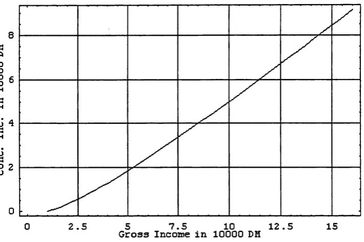
Following our general approach, we allow the penalty scheme F(h, y, p) to be de­ pendent on undeclared income h, true income y and the policy parameter p. Thus the specific penalty described by our general penalty scheme can depend on the amount of non-reported income and on the evaded tax as well, which were the specifications of Allingham & Sandmo [1972] and Yitzhaki [1974], th at proved to be crucial for the results. Furthermore, this general representation allows for an income-dependent penalty which is quite common for real tax systems. Examining existing penalty schemes more closely we see th at usually two components determine penalties for tax evasion: income and a measure for the severity of the offence. The amount of tax the taxpayer tries to evade (denoted by Te) or the amount of concealed income h are the two natural possibilities for the latter. Following the observation th at the income and severity parts are multiplicatively combined in real world tax laws, we can write:

F ( h, y, P) = y(y, P) • /(T e, P) or (26) = 9( y , P ) - f ( h , P )

used.30 If we denote the product of the constant proportionality factors with /(/?),

we can sum up potentially fair tax systems in table 2.1.

component with income without income evaded tax

concealed income

m - V - T e f(P) ' V' h

m - T e m ■ h

Table 2.1: Potentially fair penalty schemes

Our second condition for a fair penalty scheme is th a t the proportionality factor /(/?), which is the same for all taxpayers should be chosen the way th a t detected tax evasion does not lead under any circumstances to a negative ex post net income. That means th at y — t(y)y — F(h, •) > 0 has to hold for all income levels and all evasion levels.

component with income without income

evaded tax concealed income

m < ( l - t ) / ( t y ) m < { l - t ) / y

Table 2.2: Fair penalty factors

Table 2.2 reports the maximal proportionality factors to assure th a t the con­ dition above is fulfilled. Upper bars denote maximum values in the population.31

Using the conditions imposed above we can state the following definition for a “fair” penalty scheme.

30 These properties are widely observed in real world tax system s as far as m onetary penalties are concerned. The latter restriction may not hold for the degree of severity, when the penalty becomes imprisonment. For simplicity reasons we do not consider those discontinuities of penalty schemes.

D e fin itio n 2.4.2 A penalty scheme is called fair if it has the following properties: 1. It never leaves the taxpayer with negative ex post period income.

2. Its severity of offence component is proportional to the evaded tax or to the concealed income.

3. I f it has an income component, the income component is proportional to the gross income.

4. I f it has an income component the income component is multiplicatively combined with the severity of offence component.

Evasion costs

In specifying the evasion cost we stick to the definition we made above. In ad­ dition, we add the policy parameter to its arguments, since some governmental action may have an influence on the evasion cost. We assume the evasion cost to be growing with non-reported income. The marginal evasion cost is non-decreasing in the in­ come non-reported. The costs further depend on the gross income and on the evasion opportunity. By definition evasion costs fall with an increasing evasion opportunity. We can write the evasion cost as C(y,h,9,/3) according to our assumptions:

S > °- S>°

<27>

f < o VS (28)

should decrease in our continuous approximation with a rising income for all levels of evasion, because the cheapest means of evading can be used to evade a bigger amount. The other extreme is th at the new source of income has a higher marginal evading cost than all old sources of income. Then there is no change in the marginal cost of evading up to the old income. If the new (single) source of income lies with its marginal evasion cost somewhere in between the lowest and highest sources then the marginal evasion cost sinks for all evasion levels th at cannot be achieved with this source. Expressed in technical terms with respect to the undeclared income we get:

Q2 C

< 0

VM

dhd9

For convenience we define a typical average evasion cost function. The assump­ tion th a t a higher income does not systematically more likely stem from a certain source leads to the conclusion th at on average the new income rises equally for the different income sources. The counterpart - in terms of an evasion cost function - is a marginal concealment cost, th at depends somehow on the share of non-reported in­ come to gross income. So our evasion cost function of section 2.2 could be a typical average evasion cost function. To allow for cost functions of different steepness we use a parameter 7 as exponent which has to be larger than one. Policy influences are

(30)

2.4.2

O ptim al reported income

Putting all the parts together we can write down the expected income, conditional on the amount of undeclared income:

E ( K •) = ( ! - p ) [ y - ( y - h ) - K v - h> •)] - P F ( h , •) - C { h , •) (3i)

Having set up the general model, we can state the first-order condition for individually optimal non-reported income:32

E h = ( 1 - p ) T d - p F h - C h = 0 (32)

We assume th at this condition can be met: this means th at we have a local extremum for at least one taxpayer. To check whether we get an interior solution, th a t maximizes the expected value of the taxpayer, we have to look on the second order condition. We obtain always an interior solution and a maximum, whenever the second derivative is globally negative.33 The second order condition is:

Ehh = - ( 1 - p)Tdd - pFhh - Chh < 0 (33)

Tdd is non negative if we assume a globally non-regressive tax system, since it is just

the second derivative of the tax liability. It could only be negative if the marginal tax

32 Subscripts denote partial derivatives. Using the Tax liability T is convenient to abbreviate the notation.

33 A further necessary condition is that there exists a taxpayer with sufficiently low fixed evasion costs «. This is assumed in the following analysis.

D efin itio n 2.4.3 A typical average evasion cost function has the form K1

liability were falling. But this would violate the condition for a globally non-regressive tax system. In the following we will restrict ourselves to globally non-regressive tax systems, and hence the first term has to be non-positive. The second term is non­ positive if the penalty rises proportionally or more than proportionally with the not declared income, i.e. the marginal penalty is not decreasing with concealed income. The third term is negative, since the evasion costs rise more than proportionally with the concealed income. In conclusion we can say th a t for a penalty scheme, where the penalty is at least proportional to the unreported income, the extremum found by the first-order condition is a maximum. A unique solution is obtained, since the optimization problem is globally convex in th at case. Even for a penalty system th a t has falling marginal penalties the optimization problem is well behaved if the curvature of the evasion cost dominates the curvature of the penalty function. In the following we assume an interior solution.

If we examine the first-order conditions for the different fair penalty schemes, we see th at the necessary conditions for an interior solution are th at, on the one hand, the tax system is such th at the taxpayer faces a better than fair gamble, and on the other hand, the evasion costs are growing fast enough to prevent the taxpayer from becoming a ghost. The latter condition is assumed to be fulfilled in general. The (global) fair gamble conditions for the different penalty schedules are shown in table 2.3. The dependence of / on (3 is omitted.

component with income without income evaded tax

concealed income

i - p - f -p y > o

(1 - p ) T d - f - p- y > 0

1—p — f p > 0

(1 - p)Td - f • p > 0 Table 2.3: Global fair gamble conditions for fair penalties

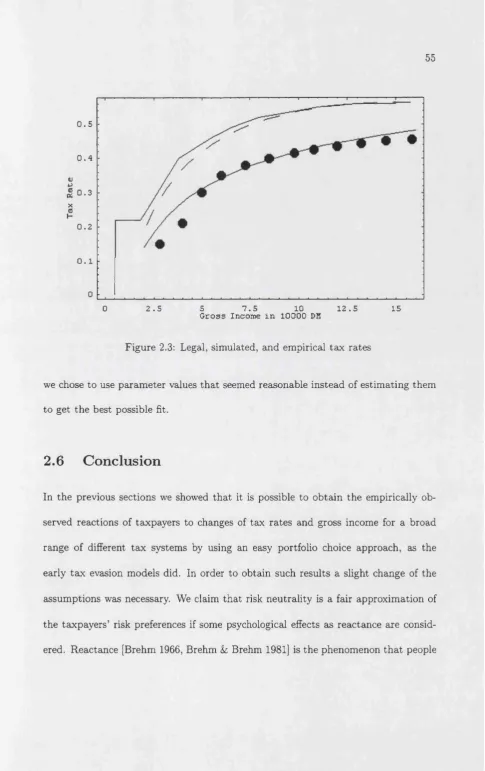
penalty schemes. They are shown in table 2.4. Since Chh is positive and Tdd is non­ negative (under the assumption of a non-regressive tax system), the second order conditions for a maximum are always met if the fair gamble condition holds.

component with income without income

evaded tax concealed income

—Chh - Tdd(l - p - f - p - y )

—Chh — (1 —p)Tdd

—Chh ~ Tdd{ 1 —p — f mp)

—Chh — (1 — p)Tdd

Table 2.4: Second order conditions

This leads to the following proposition.

P r o p o s itio n 2.4.1 Under a non-regressive tax system, a fair penalty scheme, suf­ ficiently low fixed evasion costs, and sufficiently fast growing typical average evasion

costs we obtain a unique, interior solution for the maximization problem.

2.4.3

Changes in gross incom e

Assuming th a t the conditions for an interior solution hold we are able to examine the effects of policy changes and changes in income. The evaded tax is given by the equation:

Differentiation with respect to y leads to

where dh* / d y represents the change of the optimal non-reported income due to a change in gross income. We see th at dh*/dy > 0 is a sufficient condition for a higher gross income to lead to a higher amount of taxes evaded. The reason for this fact is th at a non-regressive tax system implies d T( y ) / dy > dT(d)/dd. We have to determine the sign of dh*/dy, which is given by:

— f ~ p)Tdd — Oyh ~ pFyh (35)

dh

dy h=h" Ehh A

»

The second derivative of the objective function (i.e. Ehh) is denoted by A. Since —A is positive, we only have to look at the sign of Eyh- We know th a t ( 1 —p)Tdd, which

is the incentive to evade in order to get a lower tax bracket for rising income, is non negative. The mixed derivative of the typical cost function used here is negative - and so — Chy is positive. The value of the mixed derivative of the penalty scheme Fyh, can be interpreted as the change in the marginal penalty due to an increasing

income, and depends on the specification. A closer examination leads to the following proposition.

P ro p o s itio n 2.4.2 Under a non-regressive tax system a taxpayer with a typical average evasion cost function will evade more taxes when his gross income rises,

if the fair penalty scheme has no income component I f the fair tax system has

average evasion cost function for realistic detection probabilities and tax rates will

evade more taxes when her gross income rises even i f the system is least favourable

for evasion.

P r o o f See appendix. ■

2.4.4

P olicy effects

After checking the conditions for a higher gross income leading to more tax evasion we now examine the effects of policy changes on tax evasion. Since the effects of higher audit probabilities p and higher fines - i.e. an increased / - are not very interesting and lead to the intuitive result of less tax evasion, we concentrate on changes in the tax system and the evasion opportunity. We again restrict our attention to non-regressive tax systems, fair penalties and typical average evasion costs.

Changes in the tax system

A policy change affecting the tax laws is expressed by a change in the policy parameter (3. Here we assume that such a policy change does not influence the evasion opportunities and the evasion costs, i.e. Chp = 0. But since the penalty for detected tax evasion may depend on the tax rates, the effective penalty can be changed by a change in the tax law.

The effect of a policy change is given by:

dh w h=h'

—

Since we know th at the second derivative of the objective function is negative, it is sufficient for determining the sign of equation 36 to find the sign of E^p- If we restrict ourselves to the fair penalty schemes defined above, we can report (in table 2.5) the mixed derivatives for the schemes based on evaded tax Te or concealed income h, respectively with or without income components.

com p onent with income without income

evaded tax concealed income

(i - v - f p y ) M O + d*td0(d*)\

(1 - p) M O + d*td0{d*)\

(1 “ P ~ f P) M O + d*td0(d*)]

(1 - p) M O -f d*tdp(d*)] Table 2.5: Effects of policy changes

In the case where the evaded tax Te is the measure for the severity of the offence the first term in brackets (for systems with or without income component) is positive, because it is just the fair gamble condition from table 2.3.

For the case where the concealed income is the measure the term ( 1 — p) is

obviously positive as well. We see th at the sign of equation 36 for fair penalty schemes only depends on the sign of [tp(d*) + d*tdp(d*)\, which is just the cross derivative of the tax liability for the formerly optimal income declared (denoted Tdp{d* ) ) 34 If we postulate th a t the change does not lead to a regressive tax system we know th a t for an increase of the average tax rate (i.e. tp(d) > 0) the change in the marginal tax

liability (Tdp{d)) has to be positive as well. The interpretation of this finding is given in the following proposition.

P r o p o s itio n 2.4.3 A change in a non-regressive tax system with a fair penalty scheme, which leaves evasion opportunities unchanged and results in another non-

regressive tax system, leads to a taxpayer concealing more income if the average tax

rate at his formerly optimal declared income rises.

Tax evasion due to changes in the tax system is promoted by two things - average tax rates and progression. The former influence - if average tax rates rise - dominates the latter in non-regressive tax systems. T hat means th at for example a tax reform which results in higher average tax rates induces more tax evasion, even when the progression is lowered. The opposite conclusion is not necessarily true. A reform leading to a lower average tax rate for a taxpayer at his formerly declared income, but to a higher progression as well does not necessarily induce less concealed income.

Effects of changes in the evasion opportunities

W ith the typical average evasion cost function we get

= (37)

If the policy reduces the evasion opportunity (6p < 0) the expression above is nega­ tive. The taxpayer will report more income. For a policy th a t makes evasion easier (6/3 > 0) we get a positive sign, and consequentially more tax evasion.

P r o p o s itio n 2.4.4 For a typical average evasion cost function, a policy that reduces (improves) evasion opportunities leads to less (more) tax evasion.

2.5

Sim ulating the German ta x system

A recent paper [Lang et al. 1997] estimated the extent of income tax avoidance and evasion for the case of Germany. They used individual income d ata for the year 1983. Amongst other things they estimated the resulting effective marginal tax rates after avoidance and evasion. It is now possible to compare the results they got empirically with the results a simulation of our proposed model provides. Since the German 1983 tax tariff was not continuous and differentiable, first of all, the system has to be approximated with a continuous and differentiable function. A reasonably good approximation for the marginal tax rate T'(y) in the 1983 tariff is:

T'{y) = 0.0152 - 0.0201y + 0.3139 log y

incomes. Since it makes not too much sense to deal with negative marginal tax rates

(from our approximation function), we exclude gross incomes below 10,000 DM.

0.4

<u 4J

0

u X <c

4-> —I

<c a

• H

Ol I

0 2.5 5 7.5 10 12.5 15

Gross Income in 10000 DM

Figure 2.1: The 1983 tax system and its approximation

In our model we work with average tax rates rather than with marginal tax

rates. To obtain the average tax rate function we have to integrate the approximated

marginal tax rate function and to divide the resulting tax liability function by the

income y. This calculation leads to the average tax rate function:

t{y) = -0.2987 - 0.01005?/ + 0.3139logy

As a penalty scheme in Germany a system with an income and a severity component

for the simulation has the following form:

F = f - y - T e

Since the data in the empirical estimation were not sufficient to distinguish between tax evasion and avoidance, we have to use a rather moderate penalty factor th at takes into account th a t the penalty factor for avoided taxes is close to zero. A reasonable value for / is somewhere in the range between 10~ 5 and 10-7 . We used / = 10-6 .

This can be interpreted th at someone with one mil