Calibrating Remotely Sensed Ocean Chlorophyll Data: An Application of the Blending Technique in Three Dimensions (3D)

ISSN Online: 2161-7392 ISSN Print: 2161-7384

Calibrating Remotely Sensed Ocean Chlorophyll

Data: An Application of the Blending Technique in

Three Dimensions (3D)

Mathias A. Onabid

Department of Mathematics and Computer Sciences, Faculty of Sciences, University of Dschang, Dschang, Cameroon

Abstract

In this article, the extension to three dimensions (3D) of the blending technique that has been widely used in two dimensions (2D) to calibrate ocean chlorophyll is sented. The results thus obtained revealed a very high degree of efficiency when pre-dicting observed values of ocean chlorophyll. The mean squared difference between the predicted and observed values of ocean chlorophyll when 3D technique was used fell far below the tolerance level which was set to the difference between satellite and observed in-situ values. The resulting blended field did not only provide better pre-dictions of the in situ observations in areas where bottle samples cannot be obtained but also provided a smooth variation of the distribution of ocean chlorophyll through-out the year. An added advantage is its computational efficiency since data that would have been treated at least four times would be treated only once. With the ad-vent of these results, it is believed that the modelling of the ocean life cycle will be-come more realistic.

Keywords

In-Situ, 3D-Blending, Satellite, Over-Relaxation Method, Calibration,

Remotely Sensed Data

1. Introduction

The ocean environment can be considered as a continuous physical system subject to changes depending on atmospheric and weather conditions. To describe changes in a continuous physical system, there is a need to study partial differential equations. [1]

and [2] who have done much work on representation of physical systems using partial differential equations (PDE) make it clear that all physical systems exist in three space dimensions, and that representations in one or two space dimensions entails a large degree of approximations. It is on this basis that this research was motivated. Therefore

How to cite this paper: Onabid, M.A. (2017) Calibrating Remotely Sensed Ocean Chlorophyll Data: An Application of the Blending Technique in Three Dimensions (3D). Open Journal of Marine Science, 7, 191-204.

http://dx.doi.org/10.4236/ojms.2017.71014

Received: October 21, 2016 Accepted: January 22, 2017 Published: January 25, 2017

Copyright © 2017 by author and Scientific Research Publishing Inc. This work is licensed under the Creative Commons Attribution International License (CC BY 4.0).

in this research, the two dimensional blending technique that was implemented by [3]

in the case of predicting Sea Surface Temperature (SST) and also used by [4] who pio-neered the calibration of Ocean Chlorophyll, is extended to three-dimensions (3D). The inspiration for this is that, since the in situ field is expected to have a smooth relation-ship with satellite as one move from one location to another, this smoothness may also apply across time (day of data collection) since the data fields run throughout the year. Thus time was seen as a possible additional dimension which could influence the rela-tionship between satellite and in situ data fields. The idea of including time as a third variable had been proposed and implemented by [5] in their attempt to calibrate re-motely sensed ocean chlorophyll-a data using the non-parametric approach of penal-ized regression spline described by [6]. In another instance, [7] also suggested the ex-tension of the blending technique to three dimensions in order to render it more realis-tic. With the inclusion of time as a third variable, the blending problem now becomes a three-dimensional problem.

To perform the three-dimensional blending will require that the data fields are ex-tracted in three-dimensions. In order to achieve this, data are required throughout the period of a year. Extraction and processing of the data were done using latitude, longi-tude and time (averaged over weeks) as variables for both the satellite and in situ fields, following the same procedure as in the two-dimensional case described in [8]. Using the successive 8-day interval approach, the year has 46 weeks. Thus the dimensions of the extracted working fields were 241 67 46× × . The external latitudes and longitudes

that had very few or no observations were removed, leaving a real working area of

230 65 46× × . After extraction, the number of observations in the in situ field was 3999,

and after some pre-processing the number dropped to 3450, the others being identified by the satellite as land. The total number of points in the working arena is 687,700, out of which 374,164 points are on the sea surface, with the in situ observations contribut-ing only about 0.9% of the total observations in the ocean area.

2. The Blending Procedure

During the blending process, we employ the use of the partial differential equation (PDE) in three-dimensions. This was necessary since the intension was to perform blending in three dimensions. This was achieved by introducing the time variable as the third dimension. By doing this, the belief is that the resulting blended field will be a better predictor since it is expected that chlorophyll concentration could also vary as the seasons or times of the year changes.

The general linear equations governing physical fields take the form:

2 2 2

2 2 2

U U U U U

B C D E

x y x y

x y

A∂ + ∂ + ∂ = ∂ + ∂ +FU G

∂ ∂ ∂ ∂

∂ ∂ + (1)

where U is the final blended field. From here the various types of PDE (that is; Para-bolic, Elliptic and Hyperbolic) can be formed by attributing values which may be nega-tive, positive or zero to each of the parameters from A to G.

the Laplace’s equation. This is a special case of the Poisson equation and it arises when all the terms on the right hand side of the Poisson equation equal zero. The prototypical elliptic equation in three dimensions is the Poisson equation of the form:

(

)

2 2 2

2 2 2 , ,

U U U

x y z

x y z

ρ

∂ ₊∂ ₊∂ ₌

∂ ∂ ∂ , (2)

where the source term ρ is given. Thus, if this source term is equal to zero, the equa-tions become Laplace’s equation. The cross product term is not included because there is no theoretical foundation to expect convergence in such a case as seen in [10]. [3], who used the Poisson equation in the analysis of Sea Surface Temperature, stated that the advantage of the Poisson equation lies in its mode of solution and it also has the important benefit of behaving well numerically. Thus, when the equations are ex-panded by finite differencing into a set of linear algebraic equations, they can be solved iteratively to obtain a unique solution. This behaviour is especially convenient since the set of equations varies as the boundary points respond to changes.

Since the resulting matrix arising from this finite-differencing is sparse, it can be solved easily using the successive over-relaxation method. A somewhat more physical way of looking at the method, which also enhances convergence, is by making use of the diffusion equation. Therefore writing Equation (2) as a diffusion equation, with t as the time-step, the following equation is obtained.

(

)

2 2 2

2 2 2 , ,

U U U U

x y z

t x y z

ρ

∂ ₌∂ ₊∂ ₊∂ ₋

∂ ∂ ∂ ∂ . (3)

As t→ ∞, the solution to this problem is a solution to original elliptic Equation (2).

Equation (3) can then be represented using finite differencing as:

(

)

1

, , , ,

1, , 1, , , 1, , 1, , , 1 , , 1 , , , ,

2 6

n n

i j k i j k

n n n n n n n

i j k i j k i j k i j k i j k i j k i j k i j k

U U

t

U U U U U U U tρ

+ + − + − + − = ∆ + + + + + + − − ∆ ∆

where ∆ represents the difference between two points in either the i, j or k

direc-tions and ∆t represents the time-step from one iteration to another. The solution of

the system of linear simultaneous equations, resulting from this expression when all the boundary conditions have been applied, can be obtained by the over-relaxation method.

[11] has established the procedures for obtaining the stability criterion and the over- relaxation parameter which are the two determinant elements used in facilitating con-vergence to the solution when solving PDEs by the successive over-relaxation (SOR) method in three dimensions.

After having obtained the stability criterion and the over-relaxation parameter for the three-dimensional case, the Gauss-Seidel scheme for solving the system of simulta-neous equations resulting from this can be written in its extrapolated Liebmann form as follows:

(

)

1 1 1 1

, , , , 1, , 1, , , 1, , 1, , , 1 , , 1 , ,

2 , , 1 6 6 . 6

n n n n n n n n n

i j k i j k i j k i j k i j k i j k i j k i j k i j k

i j k

U U α U U U U U U U

As seen in [12], this can be written in short form as

1

, , , , , ,

n n n

i j k i j k i j k

U + =U +

α

where

1) 2

, , , , , ,

n

i j k i j k i j k

R =∇U −

ρ

limit

ε

U

∇ is calculated from the recently obtained U as 2 1 1 1

, , 1, , 1, , , 1, , 1, , , 1 , , 1,

n n n n n n

i j k i j k i j k i j k i j k i j k i j k

U U+ U−+ U + U +− U + U + −

∇ = + + + + +

2) The superscript n is the iteration number, while 3)

α

This scheme is then iterated until convergence is attained. The convergence set thus obtained is the blended field of the process. [13] provides some guidelines on how to build computer codes to solve systems of algebraic equations. Meanwhile a general idea of how to write programs in Fortran is provided by [14] while [15] provides an engi-neering approach to Fortran programming. Program written were then interfaced in the R programming environment for statistical analysis and graphical display of the re-sults obtained. [16][17][18] were used as guides to writing the R-codes.

3. Blending in 3D

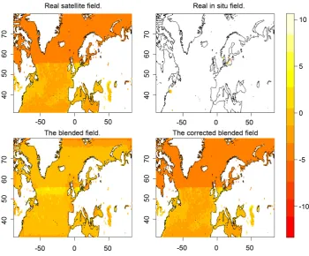
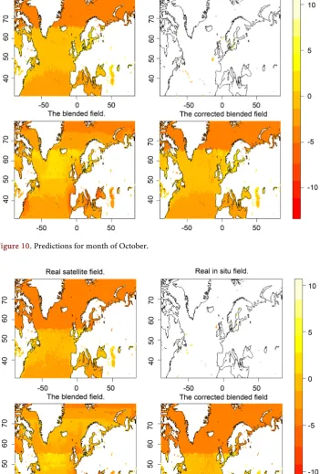
Following the procedure for solving the three-dimensional PDE using the relaxation method as described in [12], the blending process was carried out using the observed data fields. In addition [8] had shown that the “corrector factor” method performs bet-ter than the original blending technique in the prediction of ocean chlorophyll, hence this technique was also employed. The image plots in Figures 1-12 show the distribution

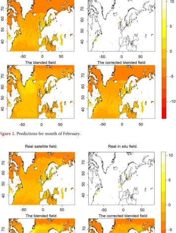
Figure 2. Predictions for month of February.

Figure 3. Predictions for month of March.

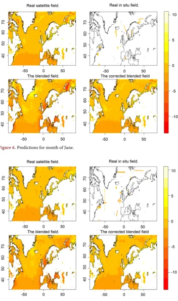
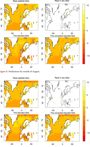
of chlorophyll density from the satellite, in situ, the normal blended and corrector fac-tor blended fields for the twelve months of the year using the 3D blending method.

Figure 4. Predictions for month of April.

Figure 5.Predictions for month of May.

Figure 6.Predictions for month of June.

Figure 7. Predictions for month of July.

Figure 8.Predictions for month of August.

Figure 9. Predictions for month of September.

Figure 10.Predictions for month of October.

Figure 11.Predictions for month of November.

Figure 12. Predictions for month of December.

4. Validating the Performance of the 3D Blending Technique

The resulting blended field from both the original blending method and the correc-tor faccorrec-tor blending method were then subjected to a validation study to assess their ability to predict the observed in situ chlorophyll. Randomly selected test sets each of size 500 were taken from the in situ field. The remaining field is then introduced into the blending process. The box plots in Figure 13 show the range of the mean squared differences between predictions from both methods and the observed in situ

values.

The range of the mean squared differences between the real satellite and in situ fields in the samples is also plotted to give an indication of the improvements provided by both processes.

From the validation study, it is clear that the resulting blended field from the correc-tor faccorrec-tor method is still the best even in the case of the three dimensional blending. To prove its power of prediction over the original blending method, the corrector factor predictions were much closer to the observed in situ values than the predictions from the original blending method though both methods show a great improvement on the prediction of in situ as opposed to the raw satellite field. The codes for running the validation study and plotting of the results were written in R as developed by [19].

5. Comparing 2D and 3D

Figure 13.A box plot of the mean squared difference between predicted and observed in situ

values from both the normal blending and the corrector factor methods using blending in three- dimensions; this can be compared with the corresponding box plot from the differences between the observed satellite and in situ samples.

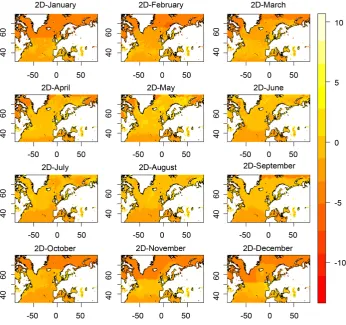
to be compared with monthly blended fields obtained from the two-dimensional blending. The images are shown in Figure 14 and Figure 15. Recall that the data fields in three dimensions contain data for the whole year divided into 46 weeks. Hence the selection of monthly data is based on the weeks that fall in the middle of the month and not on monthly averages. Since the selected data fields are maintained for both proc-esses, the effect is expected to be the same. Data used for the two-dimensional blending here were extracted from the three dimensional data fields according to the selected weeks described above. The images plotted here are from the three-dimensional blended field selected according to the weeks chosen to represent each month in the two-dimen- sional blending.

Figure 14. Predictions from the 2D blending technique.

the whole year. Thus the effects of the observed values cut across the whole year result-ing in a smooth transition from month to month. This can be seen from the gradual change of colour within and between the monthly plots. A trend can be seen with re-spect to the density of chlorophyll throughout the year. Lower values are seen during the winter and autumn periods with higher densities in spring and summer as expected.

6. Conclusions

In this research, the blending technique traditionally used in two dimensions to predict ocean chlorophyll concentration in areas where ship and buoy could not obtain values has been successfully extended to three dimensions. This was based on the fact that most physical and environmental problems exist in three dimensions, thus representing blending procedure in three dimensions would render it more realistic. The “corrector factor” method which was shown by [8] to be a better way of implementing the blend-ing technique was used. The resultblend-ing blended field did not only provide better predic-tions of the in situ observations in areas where bottle samples could not be obtained but also provide a smooth variation of the distribution of ocean chlorophyll throughout the year.

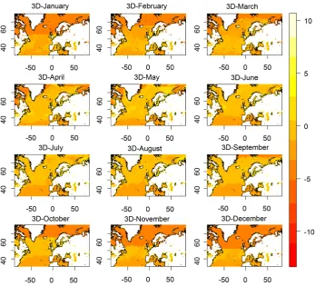
Figure 15.Predictions from the 3D blending Technique.

be used will simply be done once by employing the three-dimensional technique. Apart from this computational advantage, the physical advantage was seen when predictions over a year’s period were made using both the two and three-dimensional blending.

Another advantage of the three-dimensional blending over two dimensions is that it maintains a smooth variation between data from month to month thus providing a trend for the whole year rather than producing independent monthly or quarterly trend which is obtained when using the two-dimensional technique.

This implies that the three-dimensional blending method can serve as a better ap-proach to the blending procedure in particular and to all other processes which employ the use of the elliptic partial differential equations in their operations. With the advent of these results, it is believed that the modelling of the ocean life cycle will become more realistic.

7. Future Work

The improvement realised by the 3D Technique could be made more realistic by in-troducing the penalised technique. This could render these results more accurate as shown by [7].

References

[2] Ames, W.F. (1972) Numerical Methods for Partial Differential Equation. 2nd Edition, Thomas and Sons Limited, Port of Spain.

[3] Reynolds, R.W. (1988) A Real-Time Global Sea Surface Temperature Analysis. Journal of Climate,1, 75-86. https://doi.org/10.1175/1520-0442(1988)001<0075:artgss>2.0.co;2

[4] Gregg, W.W. and Conkright, M.E. (2001) Global Seasonal Climatologies of Ocean Chloro-phyll; Blending in Situ and Satellite Data for Coastal Zone Colour Scanner era. Journal of Geophysical Research,106, 2499-2515. https://doi.org/10.1029/1999JC000028

[5] Clarke, E., Speirs, D., Heath, M., Wood, S., Gurney, W. and Holmes, S. (2006). Calibrating Remotely Sensed Chlorophyll-A Data by Using Penalized Regression Splines. Journal of Royal Statistics Society,55, 331-353. https://doi.org/10.1111/j.1467-9876.2006.00540.x

[6] Wood, S.N. (2003) Thin Plate Regression Splines. Journal of Royal Statistical Society, Series B, 65, 95-114. https://doi.org/10.1111/1467-9868.00374

[7] Onabid, M.A. and Wood, S. (2014) Modeling Ocean Chlorophyll Distributions by Penaliz-ing the BlendPenaliz-ing Technique. Open Journal of Marine Science, 4, 25-30.

https://doi.org/10.4236/ojms.2014.41004

[8] Onabid, M.A. (2011) Improved Ocean Chlorophyll Estimate from Remote Sensed Data: The Modified Blending Technique. African Journal of Environmental Science and Tech-nology, 5, 732-747.

[9] Brandt and Diskin, B. (1999) Multigrid Solvers for Non-Aligned Sonic Flows. SIAM Journal on Scientific Computing,13, 273-501. https://doi.org/10.1137/S1064827598332205

[10] Kallin, S. (1971) Numerical Methods and FORTRAN Programming. AUERBACH pub-lisher Inc., Boca Raton.

[11] Onabid, M.A. (2012) Solving Three-Dimensional (3D) Laplace Equations by Successive Over-Relaxation Method. African Journal of Mathematics and Computer Science Research

5, 204-208.

[12] Oort, A.H. (1983) Global Atmospheric Circulation Statistics. NOAA Professional Paper 14, Nat. Oceanic and Atmospheric Administration (Silver Spring. Md.), 180 p.

[13] Edgar, S.L. (1992) FORTRAN for the ’90s Problem Solving for Scientists and Engineers. Computer Science Press, USA.

[14] Calderbank, V. (1990) Programming in Fortran. 3rd Edition, Chapman and Hall, London. [15] Forsythe, C. (1997) Contemporary Computing for Engineers and Scientists Using

For-tran90. PWS Publishing Company.

[16] Dalgaard, P. (2002) Introductory Statistics with R. Springer, Boston.

[17] Venables, W., Smith, D.M. and the R Development Core Team (2003) An Introduction to R. A Programming Environment for Data Analysis and Graphics. Version 1.8.0 Ed. [18] Wood, S.N. (2006) Generalized Additive Models: An Introduction with R. Chapman and

Hall, CRC, London.

Submit or recommend next manuscript to SCIRP and we will provide best service for you:

Accepting pre-submission inquiries through Email, Facebook, LinkedIn, Twitter, etc. A wide selection of journals (inclusive of 9 subjects, more than 200 journals)

Providing 24-hour high-quality service User-friendly online submission system Fair and swift peer-review system

Efficient typesetting and proofreading procedure

Display of the result of downloads and visits, as well as the number of cited articles Maximum dissemination of your research work

Submit your manuscript at: http://papersubmission.scirp.org/