Munich Personal RePEc Archive
Disability and Social Exclusion Dynamics
in Italian Households
Parodi, Giuliana and Sciulli, Dario
University of Chieti-Pescara
4 November 2012
Online at
https://mpra.ub.uni-muenchen.de/42445/
1
DISABILITY AND SOCIAL EXCLUSION DYNAMICS
IN ITALIAN HOUSEHOLDS
Giuliana Parodi
Università di Chieti-Pescara
e-mail: parodi@unich.it
Dario Sciulli
Università di Chieti-Pescara
e-mail: d.sciulli@unich.it
This paper investigates the dynamics of social exclusion comparing Italian households with and
without disabled people, adopting the EU definition of social exclusion and the social model approach to the disability. The analysis applies a dynamic probit model accounting for true state
dependence, unobserved heterogeneity and endogenous initial conditions to the 2004-2007 IT-SILC data. Our findings indicate that the incidence of social exclusion for households with
disable people is about double with respect to other households, and this disadvantage is especially due to exclusion in the work intensity and material deprivation dimensions. This suggests that analysis based just on income perspective could be insufficient to provide a proper
picture of reality. Second, households with disabled people are more likely to persist in social exclusion than other households. Third, persistence in social exclusion for households with
disabled people is more likely to be explained by unobserved (and observed) heterogeneity, than by true state dependence. Fourth, households with disabled members experience a stronger
severity of social exclusion, explained more in terms of structural factors than in terms of state dependence. Our findings suggest that households with disabled people could benefit more than
other households from long-term policies aimed at removing structural factors determining a social exclusion history. The severity of social exclusion, that is stronger for households with
disabled members, conforms to the same pattern.
Keywords: social exclusion, persistence, disability, dynamic probit model, initial conditions.
2 INTRODUCTION
In the last decade the interest for social exclusion has strongly increased in Europe. The
European Union designed the 2010 as the European year for combating poverty and
social exclusion, as even if EU is one of the richest areas in the world, about 20% of EU
citizens have such limited resources that they cannot afford the basics.
Various definitions of the notion of social exclusion have emerged, and all share a
multidimensional approach that proxies the individual or household well-being
extending the standard approach based on income poverty.
However, while some definitions of social exclusion (see the paragraph below), include
dimensions as civic and political participation, social interactions, health, and
education1, the EU hasbeen developing models for measuring social exclusion over the
years mainly based on economic factors.
As United Nations (2007) underlined, disability, as a factor of vulnerability, is likely to
be associated to social exclusion. This is probably true whatever definition of or
approach to social exclusion is considered and whatever is the unit of analysis, strictly
disabled persons or, in a wider view, households with disabled persons.
Approaching disability in a household rather than individual perspective is recent in the
literature of the economics of disability. Disability has an impact on the household
through multiple channels of interaction, and is mainly likely to affect the attachment to
the labour market of the household members, and the household consumption and
income. If the disabled person receives a subsidy, this increases the household income,
1 For example, the United Nations suggest to investigate social exclusion in terms of three basic
3
and therefore indirectly the household consumption. From another angle, on the
consumption side, the disabled person is likely to have additional/special consumption
requirements (She and Livermore, 2007 and 2009, Fremstad, 2009 for the USA,
Solipaca et al. 20102 for Italy, Tibble, 2005); unless these extra needs are publicly met,
the extra costs of disability affect household income, and create substitution effects on
other types of consumption. On the labour market side, the disabled person may not
work, therefore reducing the number of household members attached to the labour
market. Also, according to the severity of disability a disabled person may need care,
which can be provided by services outside the household, or within the household.
Unless care services are publicly provided, the acquisition of services draws on the
household income. Alternatively, care is provided by household members, and this
affects their attachment to the labour market (Parodi and Sciulli, 2008). Therefore it is
of interest to investigate the systemic effect that disability has on the household.
This paper focuses on the persistence in social exclusion of household which have at
least one disabled member, comparing households without disabled people (HHND)
with household with disabled people temporary limited (HHTL) and household with
disabled people permanently limited (HHD).
Jenkins (2000) describes different approaches to study the dynamics of poverty (or
social exclusion), and one of them provides for modeling the process underlying the
dynamics of poverty, paying attention to the persistence of poverty and its causes
(observable and unobservable heterogeneity and true state dependence). Literature
approaching poverty persistence using this methodology include Stevens (1999), Nolan
2 Using the Italian SILC data at regional level, they find that, standardizing by HH size, a HH with at least
4
et al. (2001), Whelan, Layte and Maitre (2001), Cappellari and Jenkins (2002),
Trivellato, Giraldo and Rettore (2002), and Poggi (2007) for social exclusion.
Most recently the literature on the economics of disability has been enriched by studies
focusing on the dynamics of poverty. This includes Meyer and Mok (2006) that study
the dynamics of individual income, consumption and earnings after a disability shock in
the US, and Shahtamaseb et al. (2011) who find that households with disabled children
in UK are not exposed to a different dynamic into and out of poverty with respect to
other households. Moreover, both Parodi and Sciulli (2012) for Italian households and
Davila-Quintana and Malo (2012) for Spanish individuals find that disability determines
a higher risk of income poverty, and explain it more in terms of persistence (initial
conditions and structural characteristics) than state dependence. It follows that this
paper adds to the existing literature introducing a multidimensional perspective to
analyzing the well-being dynamics of households with and without disabled people.
The study of persistence in social exclusion is important for its policy implications. If
social exclusion is explained by true state dependence this could suggest that short-term
policies may be effective for reducing the risk of social exclusion in the future, while if
social exclusion mainly depends on unobserved (and observable) heterogeneity,
long-term policies affecting structural variables would be effective.
Our econometric analysis is based on a dynamic probit model accounting for
unobserved heterogeneity, true state dependence and endogenous initial conditions
(Wooldridge 2005), applied to the longitudinal component of the 2004-2007 IT-SILC
database. The main findings are the following ones. First, the probability of being
socially excluded for HHD is about doubled with respect to HHTL and HHND, and this
5
dimensions. This suggests that analysis based just on income perspective could be
insufficient to provide a proper picture of reality. Second, HHD are more likely to
persists in social exclusion than other household types. Third, social exclusion for HHD
is more likely to be explained by unobserved (and observed) heterogeneity, affecting
initial conditions and persistence than by true state dependence. This is suggestive that
HHD could benefit more than other households from long-term policies aimed at
removing structural factors determining a social exclusion history.
We provide a further analysis concerning the severity of social exclusion. With this aim
we proxy the severity of social exclusion (that we interpret as a latent phenomenon)
with the number of dimensions for which an individual is socially excluded.
Descriptive findings make clear that HHD experience stronger severity of social
exclusion when compared with other household groups. Empirically, with the aim of
uncovering the determinants of the severity of social exclusion, we estimate a dynamic
ordered probit model, accounting for state dependence, unobserved heterogeneity and
initial conditions, approximating the Wooldridge’s approach provided before. The
estimation results show that for HHND and HHTL higher severity of social exclusion in
the past increases the risk of higher severity in the current period, implying the
existence of relevant state dependence. Conversely HHD experience a different pattern
with respect to the severity of social exclusion: state dependence is relatively negligible,
while we find a strong positive gradient correlation between the observations referring to the
initial period and the unobserved latent severity of social exclusion. This correlation is weaker
for the other household groups. It follows that interventions aimed at reducing the severity of
social exclusion for HHD should be focused on structural factors rather than simply rely on
6
The remainder of this paper is organized as follows. Section 2 provides definitions and
describes the data. Section 3 reports the empirical specification, while Section 4
presents the results of the econometric analysis. Finally, conclusions and policy
implications follow in Section 5.
DEFINITIONS AND DATA
We provide two basic definitions for our analysis: social exclusion and disability. The
we focus on the description of data and of the sample used in the paper.
Definition of social exclusion
Social exclusion can be seen as a process and a state that prevents individuals or groups
from full participation in social, economic and political life or as an accumulation of
confluent processes leading to marginalization with respect to the prevailing values of a
community (United Nations, 2007). A similar concept of social exclusion emerged by in
Lee and Murie (1999), while Atkinson (1999) suggested three key elements to identify
social exclusion: relativity, agency and dynamics. Other studies discuss how to
determine and to select functionings used to identify excluded individuals, and they
include as in the work by Sen and by the “Scandinavian approach to welfare” proposed
by Brandolini and D’Alessio (1998) and reinforced by Poggi (2007). Finally, Burchardt
(2000) and Burchardt, Le Grand and Piachaud (2002), include further discussions about
the way to approach social exclusion. Nolan and Whelan (2010) provide ample
reference to the literature trying to identify non-monetary deprivation in individual
7
using ECHP and EU-SILC data, with special emphasis on consumption, in order to
identify specific forms of poverty, and possible cumulative poverty.
The EU has been developing models for defining and measuring social exclusion over
the years, paralleling the debate developed especially in the UK on the inadequacies of
income as a measure of social unease (see for instance, Burchardt et al. 1999, Burchardt
et al. 2002). The Laeken European Council (December 2001) endorsed 23 common
statistical indicators of social exclusion and poverty that serve as key elements in
monitoring progress in the fight against poverty and social exclusion (the so called
Laeken Indicators). In June 2010 the European Council finally opted for a more
complex Headline Target for promoting social inclusion at EU level. The target is
defined on the basis of three indicators: the number of people at risk of poverty, the
number of materially deprived people, and the number of people aged 0–59 living in
‘jobless’ households (defined, for the purpose of the EU target, as households where
none of the members aged 18–59 are working or where members aged 18–59 have, on
average, very limited work attachment). More recently, the European Strategy 2020
adopted the same three indicators as dimensions of social exclusion3. This definition is
adopted in this article.
Specifically, social exclusion occurs if a person is socially excluded in at least one of
the three dimensions considered In terms of income, persons are socially excluded if
their equivalized disposable income is below the risk-of-poverty threshold, which is set
3 Here we concentrate on EU measurements of SE. For a UN approach, see the United Nations
8
at 60% of the national median equivalised disposable income (after social transfers)4. In
terms of work, people are socially excluded if they are living in HH with very low work
intensity, i.e. they are people aged 0-59 living in HH where the adults worked less than
20%of their total work potential during the past year. Finally, severe material
deprivation occurs for people whose living conditions are severely constrained by a lack
of resources, and experience at least 4 out of 9 of the following deprivation items:
cannot afford to pay for 1) (arrears on) mortgage or rent payments, utility bills, hire
purchase instalments or other loan payments; 2) one week’s annual holiday away from
home; 3) a meal with meat, chicken, fish (or protein equivalent) every second day; 4)
unexpected financial expenses; 5) a telephone (including mobile phone); 6) a colour
TV; 7) a washing machine; 8) a car and 9) heating to keep the home adequately warm5.
Definition of disability
The definition of disability can be tackled from several angles. The first one is based on
the International Classification of Functioning, Disability and Health (ICF, WHO,
2001), which identifies the social or inclusive model of disability, based on the
capability approach. In this respect disabled is a person whose autonomy is limited
4 The household income with different size are made comparable using the modified OECD equivalent
scale, for which the household income is normalized by an equivalent scale number (equivalent adult), where the equivalent adult is: ae=1+0.5*(adults-1)+0.3*(number of components aged less than 14). The equivalent income is Yeq=Y/ae. This system of equivalization does not take into account possible extra
weights of disabled people, necessary according to the results of the investigation by Solipaca et al. (2010)
5 Actually the EU definition refers to individuals belonging to HH. Our analysis concentrates on HH,
9
because of the characteristics of the context where she lives and operates (this is the
approach advocated by the European Disability Forum). An alternative approach is the
strictly institutional one, according to which disabled are considered the people whom
the institutional system has certified as such, and who receive some kind of disability
benefits. A third approach is the self reported one, according to which disability is
defined in terms of how people perceive their own limitations with respect to daily
activities. The three definitions have all pros and cons: in particular the second one is
open to bias determined by fraud, or by governmental choice of using disability benefits
as an instrument of financial support to poor people (for Italy see Agovino, Parodi,
2012); the third is contingent on the possible bias linked to self assessment, but also is
flexible enough to accommodate for different individual perceptions to given
limitations. Consequently, the choice of using data collected according to each system
introduces some bias in the investigation.
The EU-SILC data, which are suitable for our investigation, do not have a specific
question to identify disability, but they provide information on daily activity limitations.
It follows that the identification of disabled people with EU-SILC data is in the spirit of
the social model (Mitra, 2008), for which disability, whatever its origin may be seen as
a reduced form of the interrelations among impairment, technical help and environment
leading to activity limitations.
In our analysis we identify disabled people on the basis of two criteria, i.e. the daily
limitations in activities, and the continuity of activity limitations. We identify three
levels of limitation: no limitation, light limitation and severe limitation. The second
criterion, based on the continuity of activity limitation is stressed for instance by an ad
10
2003), where respondents were asked whether they had a longstanding health problem
or disability lasting for six months or more or expected to last six months or more
(quoted by Sloane and Jones, 2012).
The sample of analysis
Our analysis is based on the longitudinal section of the IT-SILC dataset for the period
2004-2007. The IT-SILC data is the Italian component of the EU-SILC (the European
Union Statistics on Income and Living Conditions), which provide cross-sectional and
longitudinal information. The EU-SILC collects micro-data on income, poverty, social
exclusion and living conditions from most of the EU countries in order to make
available comparable information across countries. As the EU-SILC, the IT-SILC is a
multi-purpose instrument mainly focusing on income, and devoting specific attention to
detailed income components both at household and personal level, social exclusion,
housing condition, labour, education and health.
The longitudinal component of the IT-SILC dataset includes about 105000 individuals
and about 49292 households for the whole period 2004-2007. However, since our
dynamic analysis requires a balanced panel, we only use information from households
present in each of the four waves of the longitudinal section in the period under
analysis. Moreover, because of the work intensity definition, for the sake of
homogeneity, we focus just on households where at least a household member is in
working age i.e., in our case, where at least one household member is aged 18-59 and, if
aged 18-24, is not a student. Finally, we eliminate households for which we register
missing values in the variables of interest. This selection excludes from the analysis
11
EU-SILC data provide information on both duration and seriousness of activity
limitations; therefore we organize the information collected on all individuals in terms
of type of limitation (if any) and its duration.
We acknowledge that temporary limitations, however serious, may lead to considerable
disadvantage, and therefore we identify a group of households in which at least one of
the members reports some form of limitation in some of, or even all, the years under
observation; these are defined as households with members with temporary limitations
(HHTL).
However, in this paper we use a more stringent definition of disability, i.e. we define as
disabled individuals who have experienced some form of limitation during the whole
period of observation, i.e. for the four years for which the data are available (persistence
in disability status). On the contrary, non-disabled individuals include people not
experiencing any limitation in any year under analysis, while people with temporary
limitations include those experiencing an intermediate position.
Given these premises we identify three groups of households:
- Households without disabled members (HHND);
- Households with members with temporary limitations (HHTL);
- Households with disabled members (HHD).
Within the group of HHD we consider various possible situations according to the
12
Table 1a. Identification of HHD, HHTL and HHND
0 1 2 3 4
Severe limitation
0 1496 438 197 121 61
1 66 60 62 64
-2 29 23 68 -
-3 9 66 - -
-4 73 - - -
-Light limitation Number of years of limitation
Source: our elaboration on IT-SILC data
We provide three alternative definitions of HHD according to the seriousness of activity
limitations, and their duration. Specifically we have:
a) Benchmark definition: HHD is the household in which at least one member
reports four years of activity limitations, of which at least two of severe
limitation.
b) Weak definition: HHD is the household in which at least one member reports
four years of activity limitations, whatever the seriousness of activity
limitations.
c) Strong definition: HHD is the household in which at least one member reports
four years of severe activity limitations.
The same definition of Benchmark, Weak, and Strong activity limitations apply to
HHTL as well, which are therefore complementary to HHD, while HHND is stable
across alternative definitions. According to the chosen definition of disability the groups
under investigation are the following ones (percentages are calculated over the whole
13
Table 1b. Households distribution according to the disability definition
Definition Obs. % Obs. % Obs. % Benchmark 1496 52.81% 1130 39.89% 207 7.31% Weak 1496 52.81% 1005 35.47% 332 11.72% Strong 1496 52.81% 1264 44.62% 73 2.58%
HHND HHTL HHD
Source: our elaboration on IT-SILC data
The probability of being socially excluded may vary across households according to
heterogeneous characteristics (observable and unobservable) and true state dependence,
i.e. how the probability of being currently socially excluded depends on the probability
of being socially excluded in the previous period. Observable heterogeneity is
controlled for by including the following covariates: age, gender, marital status, being
migrant, education and employment status of the household head6, as well as household
size, presence of elderly (aged more than 64), presence of children (aged 0-14), area of
residence, and employment status of the partner.
Descriptive statistics
Descriptive statistics of observable factors are reported in table 2, and provide some
preliminary information.
6 The reference person is identified according to the relpar variable included in the L07r file of the
14
Table 2. Descriptive statistics (Benchmark definition).
HHND HHTL HHD
Mean Std. Dev. Mean Std. Dev. Mean Std. Dev. Social exclusion at time t 0.208 0.406 0.288 0.453 0.488 0.500 Social exclusion at time t-1 0.211 0.408 0.283 0.450 0.475 0.500 Social exclusion at time 0 0.221 0.415 0.278 0.448 0.459 0.499 Age 46.281 10.492 53.748 12.256 62.969 11.559 Male 0.789 0.408 0.802 0.398 0.757 0.429 Consensual union 0.704 0.456 0.739 0.439 0.670 0.471 HH size 2.942 1.235 3.145 1.147 3.198 1.122 Elderly 0.069 0.300 0.301 0.592 0.771 0.772 Children 0.430 0.495 0.278 0.448 0.110 0.313 Migrants 0.024 0.154 0.026 0.159 0.005 0.069 North 0.500 0.500 0.440 0.496 0.377 0.485 Centre 0.202 0.401 0.235 0.424 0.227 0.419 South 0.298 0.457 0.325 0.469 0.396 0.489 Low education 0.414 0.493 0.577 0.494 0.765 0.424 Medium education 0.446 0.497 0.339 0.473 0.193 0.395 High education 0.139 0.346 0.082 0.274 0.021 0.143 Education missing 0.001 0.026 0.002 0.045 0.021 0.143 Employed 0.795 0.403 0.601 0.490 0.233 0.423 Unemployed 0.028 0.165 0.028 0.164 0.043 0.204 Partner employed 0.399 0.490 0.317 0.465 0.156 0.363
Source: our elaboration on IT-SILC data
With respect to social exclusion HHND and HHTL show similar incidences, while it is
much higher for HHD.
The average age of HH head increases monotonically in the three groups considered,
from 46 in HHND to 54 in HHTL to 63 in HHD. The age characteristic also explains
other demographic characteristics in the three groups; in particular, in demographic
terms, it explains the monotonical increase in the incidence of elderly people in the HH
of each of the three groups, and the comparable monotonical decrease in the incidence
of children in the HH of the same three groups.
Several personal characteristics of the HH head clearly identify HHND, HHTL, and
HHD as three distinct groups. This is the case for area of residence, with the
15
incidence of living in the South; given that self reported disability refers to ease in
performing daily activities, this can partly be explained by an environment which in the
South is less favorable to the inclusion of disabled people. In educational terms, the
incidence of medium and high education if the HH head decreases from HHNT, to
HHTL to HHD. It is also the case in employment terms, with the monotonical decrease
in the incidence of the HH head employment from HHNT, to HHTL, to HHD; this can
partly be explained by the above noted increasing age of the HH Head for the same
three groups. It is also the case for HH size, which slowly but monotonically increases
among the three groups; this may be explained by the need to share the care of disabled
members among several people; obviously an adequate provision of public service
would make the HH size less relevant. Other groups of characteristics identify strong
similarities between HHND and HHTL, compared with HHD which shows very
different values.
The incidence of unemployment is quite similar for HHND and HHTL heads, and
nearly double for HHD heads; also, for HHD the incidence of the partner being
employed is much smaller, i.e. less than half, than for the other two groups. The
considerations developed about these last three variables contribute to explain for HHD
the high value of the work intensity dimension of social exclusion as we will show in
Table 3 and 4 above.
Social exclusion and disability: descriptive evidence
Descriptive evidence provides a preliminary framework of the association between
social exclusion and disability, according to the indicators and the definitions discussed
16
from the other two groups, both in terms of incidence of being socially excluded and by
type and number of dimensions for which households are socially excluded. HHTL
usually are positioned in an intermediate position.
Looking at Table 3, just above one fifth of all HHND are socially excluded, and this
percentage monotonically increases among the three groups, as 28.5% of all HHTL are
socially excluded, and 48,07% of HHD are socially excluded.
Considering now the individual dimensions of social exclusion, Table 3 shows that: 1)
the incidence of each dimension of social exclusion increases from HHND, to HHTL, to
HHD; 2) the incidence of the income dimension of social exclusion is higher than the
incidence of other dimensions of social exclusion for HHND; 3) the incidence of the
work intensity dimension of social exclusion is close to the income dimension of social
exclusion for HHTL while for the group of HHD it reaches the very high value of
[image:17.595.86.442.495.550.2]36,59%7.
Table 3. Incidence of social exclusion among household types and by dimensions.
HH type SE SE income SE work intensity SE deprivation
HHND 21.12% 14.32% 9.38% 3.96%
HHTL 28.54% 16.11% 16.62% 6.15%
HHD 48.07% 18.24% 36.59% 12.44%
Source: our elaboration on IT-SILC data
The stronger disadvantage for HHD obviously emerges in terms of the incidence of not
being socially excluded in any dimension (Table 4, first row): it is 79% for HHND,
7 The predominance of social exclusion in the work dimension, may be partly explained by the
17
about 71% for HHTL and just 52% for HHD. Similarly, the probabilities of being
socially excluded in one, two or three dimensions are higher for HHD than for HHTL
and HHND, with the exception of the income dimension, possibly indicating a positive
role of disability benefits in reducing the risk of income social exclusion8. In this
context it also emerge that social exclusion for HHD is more likely due to the work
dimension (four times greater than for HHND), while the income dimension is
relatively less relevant. As anticipated this finding can be partly associated to the higher
incidence of elderly people in HHD. However, further explanations about the structure
of social exclusion for HHD may consist in the combined effect of disability benefit and
poor caring services for disabled people that possibly affects the labour market
participation of other household members (Parodi and Sciulli, 2008).
Finally, Table 4 also shows that, even though different dimensions of social exclusion
may intervene at the same time, exclusion in multiple dimensions is less likely than
exclusion in one dimension (e.g. social exclusion among HHD is in one dimension
33% and 15% for more than one, and other households follow quite similar patterns).
This finding is also confirmed by the correlation coefficient among different dimensions
that ranges from 0.17 to 0.26, indicating weak correlation among social exclusion
dimensions9.
8
This finding confirms Atkinson and Marlier (2010) p. 148: “In each of the 25 countries analysed here, the presence of at least one person in bad health (self-defined status) in the household seems to have no
significant impact on the risk of income poverty”.
9
18
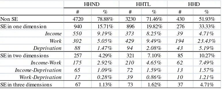
Table 4. Incidence and severity of social exclusion by household types and dimensions
# % # % # %
Non SE 4720 78.88% 3230 71.46% 430 51.93% SE in one dimension 940 15.71% 896 19.82% 276 33.33%
Income 550 9.19% 373 8.25% 39 4.71% Work 302 5.05% 429 9.49% 194 23.43% Deprivation 88 1.47% 94 2.08% 43 5.19%
SE in two dimensions 257 4.29% 321 7.10% 85 10.27%
Income-Work 175 2.92% 210 4.65% 62 7.49% Income-Deprivation 65 1.09% 72 1.59% 13 1.57% Work -Deprivation 17 0.28% 39 0.86% 10 1.21%
SE in three dimensions 67 1.13% 73 1.62% 37 4.71% HHND HHTL HHD
Source: our elaboration on IT-SILC data
Three main considerations emerge. First, the income support received by HH with
disabled people appears to succeed in protecting their incomes against being socially
excluded only in terms of the income dimension of social exclusion, and this protection
is more successful for HHD. Second, income support appears to protect HHD from the
income dimension of social exclusion, but much less so from the deprivation dimension
of social exclusion. This suggests that the consumption needs of HHD are not
sufficiently taken into account by the policy instruments geared at supporting HH with
disabled people: support income received by HH with severe disabilities appears just
sufficient to pay for the extra needs of their disabled members, and the HH cannot
therefore afford the consumption goods to which the deprivation dimension of social
exclusion refers to. Third, the work intensity dimension of social exclusion has high
values for HHD.
The number of dimensions in which the household is socially excluded is interpreted as
a proxy for the latent phenomenon of the severity of social exclusion. At descriptive
19
of HHD socially excluded in one dimension is 33.3% against 19.8% for HHTL and
15.7% for HHND. Social exclusion in two dimensions is experienced by 10.3% of
HHD, 7.1% of HHTL and 4.3% of HHND, while being socially excluded in all three
dimensions is experienced by 4.7% of HHD, 1.6% of HHTL and 1.3% of HHND. An
empirical analysis on the severity of social exclusion is provided below.
Dynamics of Social Exclusion and Disability: descriptive evidence
Evidence emerging from Table 5 (number of years in social exclusion) points in the
same direction and adds new information. The percentage of households that have been
never socially excluded represent 64% of HHND, 56% of HHTL and just 34% of HHD.
The incidence of being socially excluded in one year is very similar for all households,
while the incidence of being socially excluded during two or three years is higher for
HHD than for other household types. Finally, the incidence of being socially excluded
along four years, i.e. all years under analysis, is 31% for HHD: respectively two and
three times more than for HHTL and HHND. This points in the direction of a stronger
[image:20.595.84.430.581.686.2]persistence in social exclusion for HHD.
Table 5. Social exclusion by number of years and household types
HH socially
excluded Obs. % Obs. % Obs. % Never 957 63.97% 635 56.19% 71 34.30% Only 1 year 194 12.97% 125 11.06% 25 12.08% 2 years 117 7.82% 118 10.44% 25 12.08% 3 years 76 5.08% 79 6.99% 21 10.14% 4 years 152 10.16% 173 15.31% 65 31.40%
HHND HHTL HHD
20
The previous evidence is confirmed from information from Table 6, where we show
both the correlation coefficient between social exclusion at time t and t-1 and the
transition matrix. Interestingly, the correlation coefficient is very similar across
household types, while the transition probabilities in the main diagonal (persistence)
quite strongly differ across households. Specifically, the probability of remaining in not
social exclusion is 73% for HHND, 65% for HHTL and just 43% for HHD while, on the
contrary, the probability of remaining in social exclusion is much higher for HHD
(39%) than for HHTL (22%) and HHND (15%).
The causes of this evidence are more deeply investigated by the econometric analysis.
Table 6. Social exclusion dynamics: correlation coefficient and transition matrix
t-1 \ t Not SE SE Not SE 72.79% 6.13% SE 6.39% 14.68% Not SE 64.57% 7.17% SE 6.64% 21.62% Not SE 43.00% 9.50% SE 8.21% 39.29%
Correlation matrix Correlation
coefficient 0.622 0.661
0.646 HHND
HHTL
HHD
Source: our elaboration on IT-SILC data
THE ECONOMETRIC MODELS
A dynamic probit model
The probability of a household being social excluded is estimated by applying a
dynamic probit model accounting for both unobserved heterogeneity and true state
dependence. The introduction of the lagged social exclusion indicator among the
covariates allows us to identify the presence and the magnitude of the state dependence
21
(1) seit seit xit i uit
' 1 *
with i = 1,…,N indicating the cohort-member and t = 2…T the time periods. xit is a
vector of explanatory variables, β is a vector of unknown parameters to be estimated, αi
is the individual specific unobserved heterogeneity and uit is the idiosyncratic error term.
We assume that both αi and uit are normally distributed and independent of xit and that
there is not serially correlated in uit. Finally, seit* is the latent dependent variable and seit
is the observed binary outcome variable, seit-1 is the lagged social exclusion status and γ
is the state dependence parameter to be estimated. seit may be defined as:
(2) else 0 0 s if 1 it* it
e se
Specifically se takes value one if the household is socially excluded at time t and value
0 if the household is not socially excluded.
It follows that the probability of being socially excluded for household i at time t is
specified as:
(3)
seit seit xit i
seit xit i
' 1 1, ,
| 1 Pr
where Φ is the cumulative distribution function of a standard normal.
The assumption about the independence between αi and xit may be relaxed adopting the
Mundlak approach (Mundlak, 1978). This approach takes into account possible
correlation between random effects and observable characteristics, simply allowing a
relationship between α and either the time means of time-variant explanatory variables.
This implies to decompose the unobserved heterogeneity term in two parts:
(4) i xii
22
where xi represents the part of unobserved heterogeneity correlated with the explanatory
variables and i represents the part of unobserved heterogeneity uncorrelated with the
explanatory variables.
It follows that the new equation for the latent dependent variable may be written as:
(5) seit seit xit xii uit
' ' 1 *
and the probability of being socially excluded for household i at time t reads:
(6)
seit seit xit i
seit xit xiai
' ' 1 1, ,
| 1 Pr
Finally, we consider the possibility of correlation between αi and yit-1, the so-called
initial conditions problem (Heckman, 1981). We address the initial conditions problem
following Wooldridge (2005) that has proposed an alternative Conditional Maximum
Likelihood (CML) estimator that considers the distribution conditional on the initial
period value. The idea is that the correlation between sei1-1 and αi may be expressed by
the following equation:
(7) i sei zii
' 1 1 0
where ε is another unobservable individual specific heterogeneity term that is
uncorrelated with the initial social exclusion status se1. Wooldridge (2005) specifies that
zi corresponds to the xi contained in the Mundlak specification, calculated for periods 2
to T.
It follows that the probability of being socially excluded for household i at time t reads:
(8)
seit seit xit yi
i
seit xit
sei zi
i
' 1 1 ' 1 1
1, , ,
| 1 Pr
The Wooldridge approach is based on the conditional maximum likelihood (CML) that
23
conditional on the initial observations. The contribution to the likelihood function for
the cohort-member i is given by:
(9)
i iT t it i i i it it
i se x se z y g d
L
2
' 1 1 '
1 2 1
where g(η) is the normal probability density function of the new unobservable
individual specific heterogeneity.
A dynamic ordered probit model
With the aim of estimating the severity of social exclusion we adopt a dynamic ordered
probit model (see Contoyannis, Jones and Rice 2004, for an application), where the
response variable is a discrete variable taking values 0, 1, 2 and 3 according to the
number of dimensions for which the households is socially excluded. Consistently with
the above analysis we include previous social exclusion status in order to capture state
dependence. Moreover, we allow for normally distributed unobserved heterogeneity
and, drawing from the Wooldridge’s approach adopted above, we also deal with the
initial condition problem.
In the standard approach, the latent variable specification of the empirical model can be
written as follows:
it i it it
it sse x v
sse* 1 ' where i=1…N and t=2,…, Ti
To capture state dependence we include sset-1 that is a vector of indicators for the
number of social exclusion dimensions reported in the previous wave and the ηs
parameters to be estimated. θi is an individual-specific and time-variant random
component. vit is a time and individual-specific error term which is assumed to be
24
with θi. vit is assumed to be strictly exogenous, that is, the xit are uncorrelated with vit for
all t and s. In the data the latent outcome (severity of social exclusion, sse*) is not
observable, while we can approximate the severity through the number of dimensions
for which a household is socially excluded. In other words, the number of dimensions
may be thought of as an indicator of the category in which the latent indicator falls
(sseit). The observation mechanism may be expressed as follows:
j it
j-it j sse
sse if 1 * , where j = 1,…, m
where 0 ,j j1 ,m . Given the assumption that the error term is
normally distributed, the probability of observing the particular number of social
exclusion dimensions experienced by household i at time t, conditional on the regressors
and the individual effect is,
it
j it it i
j it it i
itj P sse j x sse x sse
P ' 1 1 ' 1
where Φ is the normal standard distribution function. In order to deal with the
identification of the intercept and the cutpoints (μ), the following normalization is
usually adopted: β0=0. By implementing the random effects estimator, the individual
effect is integrated out, under the assumption that its density is N(0, σθ2), to give the
sample log-likelihood function:
n i itj d P L 1 2 22 exp 2
2 1 ln
ln
The expression may be approximated by the Gauss-Hermite quadrature procedure.
When we deal with the initial condition problem following the procedure suggested by
Wooldridge (2005), the distribution of the individual effects is parameterized as
follows:
i i i
i sse w
'
25
where ο is another unobservable individual specific heterogeneity term that is
uncorrelated with the initial social exclusion status sem1. Wooldridge (2005) specifies
that wi corresponds to the average over the sample period of the observations on the
exogenous variables calculated for periods 2 to T (Mundlak, 1983).
ESTIMATION RESULTS
The probability of being socially excluded may vary across households because of
observable and unobservable factors, and because of true state dependence. In what
follows we firstly discuss the estimation results concerning unobserved heterogeneity
and true state dependence and then we focus on the role of observable factors affecting
social exclusion. Moreover, for brevity, we do not comment on the estimation results
from all dynamic probit specifications, but we mainly focus on those obtained from the
Wooldridge’s model using the benchmark definition of household with disabled
people10. However, for comparative purpose, we also comment on the estimation of the
true state dependence parameter obtained from the Mundlak model with the aim of
highlighting the differences between the assumption of exogenous and endogenous
initial conditions.
True state dependence and unobserved heterogeneity
Table 7 shows the state dependence parameters estimated by the Mundlak model,
including the marginal effects. According to these estimates the magnitude and the
significance of true state dependence is particularly strong. Specifically, being socially
excluded in the previous period increases the probability of being socially excluded in
26
the current period by 46.1% for HHND, by 58.6% for HHTL and by 61.3% for HHD.
This points in the direction of significant persistence in social exclusion, especially for
HHD, agreeing with the descriptive evidence presented above. Results from the
Mundlak model also show that unobserved heterogeneity is negligible and not
statistically significant. It follows that, assuming exogenous initial conditions, our
results reveal that state dependence strongly explain social exclusion and then policies
aimed at reducing the risk of social exclusion should be addressed at keeping
households (especially with disabled members) out of social exclusion (e.g. by
providing monetary and non-monetary transfers aimed at increasing income and
[image:27.595.86.299.416.470.2]reducing material deprivation, as well as employment measures).
Table 7. State dependence parameters estimation in Mundlak model
Coef. s.e. mfx HHND 1.574 0.062 0.461 *** HHTL 1.759 0.065 0.576 *** HHD 1.729 0.136 0.613 *** Source: our elaboration on IT-SILC data
Estimation results obtained from the Wooldridge model are showed in Table 8. As
anticipated, this specification allows us to relax the exogeneity assumption, allowing for
endogenous initial conditions. An initial condition problem arises when the start of the
observation period does not coincide with the start of the process generating social
exclusion. It follows that socially excluded households may be there at the start of the
observed period because of factors favoring social exclusion or because of an earlier
27
Estimations from the Wooldridge model differ with respect to those obtained from the
Mundlak model. Unobserved heterogeneity is statistically significant and not negligible
in magnitude, and the estimated σu is greater for HHD (1.43) rather than for other
household groups (0.94 for HHND and 0.76 for HHTL). According to the estimations
obtained from the Wooldridge model true state dependence is smaller in magnitude for
HHND and HHTL (the marginal effects are, respectively, 9.5% and 23.9%), and not
significant for HHD. This seems to be strongly explained by the role of the starting
status in social exclusion: the initial condition parameters are strongly significant and
great in magnitude. In fact, being socially excluded at time 0 increases the probability of
being socially excluded at current time by 27.7% for HHND, 41.5% for HHTL and by
81.3% for HHD. This points in the direction of a substantial correlation between the
initial condition and unobserved heterogeneity, i.e. the probability of being socially
excluded at the starting period is strongly affected by unobservable factors, and these
determine a relevant propensity to be socially excluded in the current period. This effect
is particularly strong for HHD and, looking also at the true state dependence estimates,
it suggests that measures aimed at reducing the risk of social exclusion for HHD should
be prevalently addressed at single-outing structural factors determining social exclusion
and the history of previous social exclusion.
Table 8. State dependence and unobserved heterogeneity in the Wooldridge model
Coef. Std. Err. mfx Coef. Std. Err. mfx Coef. Std. Err. mfx Lag SE 0.640 0.126 0.095 *** 0.872 0.135 0.239 *** 0.207 0.292 0.082 SE time0 1.403 0.182 0.277 *** 1.415 0.204 0.415 *** 2.643 0.567 0.813 ***
Unobserved heterogeneity
u 0.937 0.113 LR-test ρ=0 0.760 0.122 LR-test ρ=0 1.432 0.305 LR-test ρ=0
ρ 0.468 0.060 42.45 *** 0.366 0.075 18.45 *** 0.672 0.094 21.96 ***
HHND HHTL HHD
28 Covariates
We now comment the Wooldridge estimation results, and the marginal effects,
concerning structural variables affecting the probability of being social exclusion, and in
particular we concentrate on statistically significant variables, i.e. HH size, area of
residence, and also education, and attachment to the labour market of the HH head and
[image:29.595.88.512.306.598.2]his/her partner (Table 9).
Table 9. Estimated parameters in the Wooldridge model: covariates
Coef. Std. Err. mfx Coef. Std. Err. mfx Coef. Std. Err. mfx
Age -0.027 0.173 -0.003 -0.009 0.131 -0.002 -0.426 0.604 -0.170
Age square 0.000 0.002 0.000 0.000 0.001 0.000 0.004 0.005 0.002
Male 0.000 0.141 0.000 -0.003 0.145 -0.001 -0.433 0.510 -0.171
Consensual union -0.252 0.462 -0.030 1.128 0.421 *** 0.196 0.335 0.918 0.132 HH size -0.136 0.153 -0.015 -0.289 0.146 ** -0.067 -1.399 0.410 *** -0.557
Elderly -0.288 0.415 -0.032 -0.165 0.263 -0.038 0.519 0.570 0.207
Children 0.136 0.266 0.015 0.399 0.292 0.100 0.087 0.937 0.035
Migrants 1.063 0.258 *** 0.234 0.580 0.253 ** 0.171 0.670 1.908 0.253
North -0.220 0.126 * -0.024 0.027 0.116 0.006 -0.330 0.398 -0.130
South 0.621 0.136 *** 0.085 0.588 0.125 *** 0.150 0.918 0.436 ** 0.354 Medium education -0.288 0.099 *** -0.031 -0.183 0.100 * -0.041 0.654 0.390 * 0.254 High education -0.316 0.154 ** -0.029 -0.081 0.180 -0.018 0.537 0.983 0.208 Employed -2.274 0.223 *** -0.562 -2.001 0.234 *** -0.529 -1.863 0.655 *** -0.577 Unemployed -0.592 0.330 * -0.042 -0.650 0.341 * -0.105 -0.442 0.776 -0.169 Partner employed -0.683 0.221 *** -0.070 -1.110 0.216 *** -0.208 -2.729 0.994 *** -0.633 Year 2006 0.179 0.092 * 0.021 0.203 0.086 ** 0.049 -0.514 0.231 ** -0.201
Year 2007 0.161 0.120 0.019 0.076 0.094 0.018 -0.495 0.284 * -0.193
Constant -2.221 0.824 *** - -2.780 0.817 *** - -0.252 4.050
-Observations Households Wald chi2(29) Prob > chi2 Log likelihood 0.000 -1233.6 0.000 -226.3 3390 1130 623.62 0.000 -1079.7
HHND HHTL HHD
621 207 76.24 4488 1496 583.93
Source: our elaboration on IT-SILC data
The probability of social exclusion decreases with HH size, both for HHTL and, much
more pronouncedly so, for HHD. The marginal effect of reducing the probability of
29
HHD is nearly 40 times that of HHND. The chance of sharing the care of the disabled
person among more HH members is likely to increase the participation/hours worked
outside the HH of the HH members, and this contributes to reduce the work intensity
dimension of social exclusion.
The area of residence has a statistically significant impact on the probability of social
exclusion, in particular living in the South compared with the base category of living in
the Centre, increases the probability of social exclusion, more or less in the same way
for HHND and HHTL, and more pronouncedly so for HHD. The marginal effects
increase monotonically with the severity of disability: the marginal effect for HHD is
over three times that of HHND. The South of Italy is characterized by both high poverty
and unemployment, and these two variables contribute to two of the dimensions of
social exclusion, therefore the probability of social exclusion is likely to be high for HH
living in the South, whether with or without disabled members. In addition, the still
typical scarcity of social services in the South is likely to particularly affect the
possibility of labour market participation for members of HHD, and this may explain
the particularly high estimated coefficient of the probability of social exclusion for
HHD living in the South, which would reinforce the already high value of the work
intensity dimension of social exclusion. This confirms the territorial duality
characterizing the Italian economy. In any case, HHD living in the South appear to
suffer the greatest penalty. This has some policy implications: the South-Islands are the
areas of the country with the highest levels of diffusion and intensity of poverty, and
with high unemployment, therefore policies to improve the situation in these areas
would reduce the probabilities of social exclusion at least the two income and work
30
The medium or high educational level of the HH head above the base category “low
education”, significantly decreases the probability of social exclusion for HHND; it is
hardly or not significant for HHTL and for HHD. Education plays only an indirect role
in the dimensions of social exclusion, either via the income or via the work intensity
dimension. Our finding suggests that education above “low” succeeds in reducing the
probability of social exclusion either by increasing earnings, and/or the work intensity
for HHND, but hardly so for HHTL; the marginal effect of both medium and high
education is around 3% for HHND. For HHD the sign of the estimate is reversed, even
though scarcely significant, so that education of the HH head above the “low” level of
education increases the probability of social exclusion for HHD.
The covariates about the attachment to the labour market are assessed in terms of the
base category “not participating to the labour market”; they are highly significant for
most of the three groups considered. In particular, the probability of social exclusion is
reduced if the HH head is employed rather than out of the labour market; even though
also, and the estimated coefficients decrease monotonically from HHND to HHTL to
HHD; however, the marginal effect of HH head employment in reducing social
exclusion is the highest for HHD.
The covariate “unemployment of the HH head” reduces the probability of social
exclusion with respect to the probability of social exclusion for a HH head out of the
labour force, probably because of the income support received in terms of
unemployment benefits; the estimated coefficients are very similar for the three groups;
however, they are mostly of no statistical significance; the marginal effects are
monotonically increasing among the three groups: for HHD an unemployed HH head
31
social exclusion; however, the marginal effects for the covariate “unemployment” are
never significant.
As expected, the employment of the HH head partner significantly reduces the
probability of social exclusion for all the three groups considered, even though the
highest effect appears for HHD, where the estimated coefficient is over four times that
of HHND, and the marginal effect is about ten times that of HHND.
Severity of social exclusion
Tables 10 and 11 show estimates from the dynamic order probit model obtained using
the benchmark definition of disability. The model formally tests for state dependence
and takes into account the initial condition problem.
Since the ordered probit model estimates one equation over all levels of the dependent
variable, an estimated positive coefficient indicates the approximated (because of non
linearity of the ordered probit model) increase in the probability of being in a higher
category of severity of social exclusion. Conversely, the ancillary parameters refer to
the cut-points (thresholds) used to differentiate the adjacent levels of the response
variable. A threshold can be defined as points on the latent variable, i.e. a continuous
unobservable phenomena, that results in the different observed values on the proxy
variable (i.e. the levels of our dependent variable used to measure the latent variable).
Table 10 presents evidence about state dependence and the estimated coefficients for
the initial period observations introduced following the Wooldridge’s approach to the
32
Table 10. Severity of social exclusion: state dependence and initial conditions
Coef. Std. Err. Coef. Std. Err. Coef. Std. Err. Lag SE1 0.447 0.108 *** 0.790 0.107 *** 0.240 0.222 Lag SE2 0.726 0.177 *** 1.270 0.174 *** 0.665 0.347 * Lag SE3 1.339 0.331 *** 1.236 0.288 *** 0.693 0.531 SE01 1.377 0.153 *** 1.012 0.139 *** 1.924 0.368 *** SE02 1.809 0.233 *** 1.641 0.219 *** 3.215 0.592 *** SE03 2.647 0.469 *** 2.737 0.351 *** 4.666 0.855 ***
HHND HHTL HHD
Source: our elaboration on IT-SILC data
Our main findings suggest a significant state dependence for HHND and HHTL in terms of
severity of social exclusion. For HHND, a stronger severity in the previous period increases the
risk of stronger severity in the current period; for HHTL we find a similar effect, but the
positive effect of past severity on current severity is flatter for HHTL when compared with
HHND. With respect to HHD, we find a quite negligible link between the past and current
severity of social exclusion: the only significant parameter (10% level) is Lag SE2, that is lower
in magnitude when compared with other household groups. This agrees with the evidence about
social exclusion for which we did not find evidence of state dependence. With respect to the
initial period coefficients, we find a positive gradient in the estimated effects as the number of
social exclusion dimensions increases. This suggests a positive correlation between the initial
period observations and the unobserved latent severity of social exclusion. When we focus on
different household groups we note that the positive correlation is much stronger for HHD than
for other groups. This also agrees with evidence emerged above from the analysis of social
exclusion, and suggests that also the severity of social exclusion for HHD is much more
explained by unobservable factors than by state dependence.
Table 11 shows the effects of observable variables on the severity of social exclusion and the
estimates of the ancillary parameters. Cut1 is the estimated ancillary parameter measuring the
distance on the latent variable distribution between the lower value of our predictor variable
33
three dimensions). In turn, Cut2 and Cut3 are the successive ancillary parameters that
respectively measure the distance between zero/one dimensions and two/three dimensions, and
zero/one/two dimensions and three dimensions. According to our estimates, the ancillary
parameters for HHD are not statistically significant, while for HHND and HHTL they are
strongly significant and similar in values. Finally, the Rho term indicates the proportion of the
[image:34.595.87.426.288.637.2]total variance contributed by the panel-level variance component.
Table 11. Severity of social exclusion: estimated parameters
Coef. Std. Err. Coef. Std. Err. Coef. Std. Err. Age 0.072 0.131 -0.044 0.103 0.482 0.428 Age square -0.001 0.001 0.000 0.001 -0.004 0.003 Male -0.110 0.132 -0.058 0.119 -0.305 0.409 Consensual union -0.636 0.386 * 0.448 0.364 0.661 0.731 HH size -0.066 0.138 -0.262 0.123 ** -0.968 0.297 *** Elderly -0.222 0.343 -0.186 0.219 0.212 0.376 Children 0.026 0.233 0.356 0.237 -0.355 0.690 Migrants 0.938 0.234 *** 0.620 0.197 *** 0.308 1.585 North -0.236 0.122 * 0.006 0.097 -0.140 0.327 South 0.578 0.128 *** 0.531 0.101 *** 0.564 0.337 * Medium education -0.329 0.094 *** -0.209 0.083 ** 0.217 0.301 High education -0.374 0.151 ** -0.148 0.152 0.082 0.816 Employed -2.222 0.174 *** -1.822 0.168 *** -2.491 0.520 *** Unemployed -0.078 0.214 -0.109 0.228 -0.747 0.528 Partner employed -0.771 0.202 *** -0.889 0.185 *** -1.994 0.679 *** Year 2006 0.060 0.076 0.161 0.070 ** -0.485 0.163 *** Year 2007 0.037 0.093 0.050 0.077 -0.329 0.187 * Cut 1 1.781 0.771 ** 2.202 0.665 *** -0.192 3.088 Cut 2 3.908 0.780 *** 4.048 0.676 *** 2.504 3.081 Cut 3 5.851 0.803 *** 5.841 0.694 *** 4.283 3.086 Rho 0.485 0.046 *** 0.279 0.057 *** 0.625 0.069 *** Observations
LR chi2(33) Prob > chi2 Log likelihood
0.000 0.000 0.000 -1683.41 -1624.70 -406.11
4488 3390 621 1207.09 1151.72 228.58 HHND HHTL HHD
Source: our elaboration on IT-SILC data
with respect to observable variables, the evidence show that the severity of social
34
household head and his/her partner being employed reduce the risk of being socially
excluded in multiple dimensions. We find similar evidence both for HHND and HHTL,
but in those cases we find a significant contribution to the severity of social exclusion
also from the migration variable (positive sign) and the medium/high level of education
(negative signs).
It follows that interventions aimed at reducing the severity of social exclusion for HHD should
be focused on structural factors rather than simply rely on monetary transfers, that prevalently
produce short-term effects.
POLICY IMPLICATIONS AND CONCLUDING REMARKS.
This paper studies the social exclusion and its dynamics in Italy with a special focus on
the situation of HHD. In a comparative perspective with the situation of HHTL and
HHND, we analyze the 2004-2007 longitudinal component of the IT-SILC data
applying a dynamic probit model accounting for unobserved heterogeneity and
endogenous initial conditions.
Social exclusion, according to the recent approach of the EU, is defined along three
dimensions: income, work intensity and material deprivation, while we define disability
according to two criteria: limitation in daily activities (social model) and persistence of
limitation. Finally, the situation of the household is approximated by the situation of the
HH head.
Descriptive evidence show that almost 50% of HHD are socially excluded, about twice
more than HHTL and HHND, and they are disadvantaged especially in terms of
material deprivation and, overall, work intensity, while differences in terms of the
income dimension are quite negligible. This structure of social exclusion for HHD may
35
elderly people), but also by the combined effects of disability benefit and poor caring
services for disabled people. Moreover, HHD are more likely to persist in social
exclusion than other household types. Finally, the severity of social exclusion is
stronger for HHD than for other household groups.
Estimation results provide further information. Both the probability of being socially
excluded and its severity for all household types is explained by observable and
unobservable factors. True state dependence is significant for HHND and HHTL nor for
HHD, for which, instead, the initial conditions are particularly relevant to explain
persistence in social exclusion. In other words, the probability of being excluded in the
starting period is affected by unobservable (and observable) factors, that also determine
the propensity of HHD of being excluded in the current period.
This has some policy implications. In fact, while short-term policies aimed at breaking
the vicious circle determined by true state dependence (current social exclusion
increases per se the probability of future social exclusion), are potentially effective for
HHND and HHTL, but they could be quite ineffective for HHD. Instead, members of
HHD could benefit more than other households from long-term policies aimed at
36 REFERENCES
Agovino M. and Parodi G. (2011) “Civilian disability pensions as an antipoverty policy
instrument? A spatial analysis of Italian Provinces, 2003-2005”, in: Parodi G., Sciulli
D. (eds.), Social Exclusion. Short and long term causes and consequences, Verlag
Springer, Heidelberg.
Atkinson, A.B. (1999) “On the poverty measurement”, Econometrica vol. 55, pp. 749
-64.
Atkinson A. B. and Merlier E. (2010), Income and Living Conditions In Europe,
Eurostat Statistical Books, Luxembourg: Publications Office of the European Union,
2010, pp. 1-424
Brandolini, A., D’Alessio, G. (1998) “Measuring well-being in the functioning space”,
mimeo, Bank of Italy, Rome.
Burchardt, T. (2000) “Social exclusion: Concept and evidence”, in: Gordon, D.,
Townsend, P. (eds.) Breadline Europe: The Measurement of Poverty, pp. 385–406.
Policy, Bristol.
Burchardt, T., LeGrande, J., Piachaud, D. (2002) “Degrees of exclusion: Developing a
dynamic multidimensional measure”, in: Hills, J., Le Grand, J., Pichaud, D. (eds.)
37
Cappellari L. and Jenkins S. (2002) “Who stays poor? Who becomes poor? Evidence
from the British household panel survey”, Economic Journal, vol. 112, pp. 60-67.
Contoyannis P., Jones A.M., Rice N., (2004) “The dynamics of health in the British
Household Panle Survey”, Journal of Applied Econometrics, vol. 19, pp. 473-503.
Davila-Quintana C.D. and Malo M.A., (2012) “Poverty dynamics and disability: An
empirical exercise using the European Community Household Panel”, Journal of Socio
-Economics, vol. 41, pp. 350-359.
Dupré D. and Karjalainen A. (2003) “Employment of Disabled People in Europe in
2002”, Statistics in Focus, Population and Social Conditions, Theme 3, Eurostat, Paris.
Eurostat (2012), Population and Social Conditions, Statistics in focus, 9/2012.
Fremstad S., (2009) “Half in Ten: Why Taking Disability into Account is Essential to
Reducing Income Poverty and Expanding Economic Inclusion” CEPR Reports and
Issue Briefs, n. 30.
Jenkins, S.P. (2000) “Modeling household income dynamics”, Journal of Population
Economics, vol. 13 n.4, pp. 529-567.
Heckman, J.J. (1981) “The incidental parameters problem and the problem of initial