A Bayesian Approach for Stable Distributions: Some Computational Aspects

A Bayesian Approach for Stable Distributions: Some

Computational Aspects

Jorge A. Achcar1*_{, Sílvia R. C. Lopes}2_{, Josmar Mazucheli}3_{, Raquel R. Linhares}2 1_{Medical School, USP, Ribeirão Preto, Brazil}

2_{Mathematical Institute, UFRGS, Porto Alegre, Brazil} 3_{Departament of Statistics, UEM, Maringá, Brazil}

Email: *_{[email protected], [email protected], [email protected], [email protected]} Received May 1, 2013; revised June 5, 2013; accepted June 12, 2013

Copyright © 2013 Jorge A. Achcar et al. This is an open access article distributed under the Creative Commons Attribution License, which permits unrestricted use, distribution, and reproduction in any medium, provided the original work is properly cited.

ABSTRACT

In this work, we study some computational aspects for the Bayesian analysis involving stable distributions. It is well known that, in general, there is no closed form for the probability density function of stable distributions. However, the use of a latent or auxiliary random variable facilitates to obtain any posterior distribution when being related to stable distributions. To show the usefulness of the computational aspects, the methodology is applied to two examples: one is related to daily price returns of Abbey National shares, considered in [1], and the other is the length distribution analysis of coding and non-coding regions in a Homo sapiens chromosome DNA sequence, considered in [2]. Posterior summa-ries of interest are obtained using the OpenBUGS software.

Keywords: Stable Laws; Bayesian Analysis; DNA Sequences; MCMC Methods; OpenBUGS Software

1. Introduction

A wide class of distributions that encompasses the Gaus-sian one is given by the class of stable distributions. This large class defines location-scale families that are closed under convolution. The Gaussian distribution is a special case of this distribution family (see for instance, [1]), described by four parameters α, β, δ and σ. The



0, 2



 parameter defines the “fatness of the tails”, and when α = 2 this class reduces to Gaussian distribu-tions. The  



1,1





is the skewness parameter and for β = 0 one has symmetric distributions. The location and scale parameters are, respectively, and

(see [3]).



,

  





0,

 

Stable distributions are usually denoted by S_



  , ,



. If a random variable X S



  , ,



, then



, 0,1

X

Z  S_ 





 





(see [4,5]).

The difficulty associated to stable distributions



, ,

S_    , is that in general there is no simple closed form for their probability density functions. However, it is known the probability density functions of stable dis- tributions are continuous [6,7] and unimodal [8,9]. Also the support of all stable distributions is given in (−∞, ∞),

except for α < 1 and |β| = 1 when the support is (−∞, 0) for β = 1 and (0, ∞) for β = −1 (see [10]).

The characteristic function Φ(.) of a stable distribution is given by

 

 

 

1 sign tan ,

2

log for 1

2

1 sign , for

i t t i t

t

i t t i t





   



   

 _  _     _ _

 



  

 _{ }  

 _{  }

 _{     1}

   





 

(1.1) where i 1 and sign(.) function is given by

 

1, if 0

sign 0, if 0

1, if 0.

x x

x x

 

 

 

 _



(1.2)

Although a good class for data modeling in different areas, one has difficulties to obtain estimates under a classical inference approach due to the lack of closed form expressions for their probability density functions. An alternative is the use of Bayesian methods. However, the computational cost can be further exacerbated in as- sessing posterior summaries of interest.

duced by Buckle (1995) using Markov Chain Monte Carlo (MCMC) methods. The use of Bayesian methods with MCMC simulation can have great flexibility by considering latent variables (see, for instance, [11,12]), where samples of latent variables are simulated in each step of the Gibbs or Metropolis-Hastings algorithms.

Considering a latent or an auxiliary variable, [1] pro- ved a theorem that is useful to simulate samples of the joint posterior distribution for the parameters α, β, δ and σ. This theorem establishes that a stable distribution for a random variable Z defined in (−∞,∞) is obtained as the marginal of a bivariate distribution for the random vari- able Z itself and an auxiliary random variable Y. This variable Y is defined in the interval (−0.5, aα,β), when

, and in (aα,β, 0.5), when . The

quantity aα,β is given by



, 0

Z 



Z



0,



,

, ,

b

a_{ }  



 

 (1.3)

where





, min , 2 .

2

b_{ }    

The joint probability density function for random va- riables Z and Y is given by





   

, ,

1

, , exp

1 _{y y}

z z

f z y

t t                      

 z ,(1.4)

where , 1     

 



_{ }



 









1 , , , sin cos

cos cos 1

y b y

t y

y y b

                              (1.5) and X Z   

 , for 0.

From the bivariate density (1.4), [1] shows the mar- ginal distribution for the random variable Z is stable Sa (, 0, 1) distributed. Usually, the computational costs to obtain posterior summaries of interest using MCMC methods are high for this class of models, which could give some limitations for practical applications. One problem can be the simulation algorithm convergence. In this paper, we propose the use of a popular free available software to obtain the posterior summaries of interest: the OpenBUGS software.

The paper is organized as follows: in Section 2 we in- troduce a special case of the stable distributions, namely,

the Lévy distribution. In Section 3, we introduce a Bay- esian analysis for stable distributions. Two applications are presented in Section 4. Section 5 is devoted to some concluding remarks.

2. A Special Case of Stable Distributions:

Lévy Distribution

Some special cases of stable distributions are given for specified values of αand β. If α = 2 and β = 0 one has the Gaussian distribution withδ mean and variance equals to

2

2 . If  0.5 and  1 one has a Lévy distribu- tion with probability density function given by









1

3 2

2 0.5 ,

,

2 exp

f x x

x            _{ }  _ _   

   (2.1)

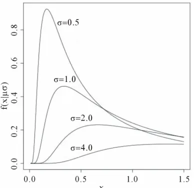
for δ< x< ∞. Figure 1 presents Lévy probability density functions for δ = 0 and different values of the σ scale parameter.

The probability distribution function of the random va- riable X with a Lévy distribution defined in (2.1) is given by









1 2 0.5 erf , , c

F x P X x

x         _    

 (2.2)

where erfc

 

x  1 erf

 

x is the complementary error function with the error erf(.) given by

 

2

0

2

erf e d .

x t

x  t





_

(2.3)

[image:2.595.327.521.513.701.2]

The Lévy distribution with probability density func-tion (2.1) has undefined mean and undefined variance but its median is given by

2 1 Median 1 2 erfc 2            _{ }  

, (2.4) a10.0705230784,

2 0.0422820123

a  ,

3 0.0092705272

a  ,

where the inverse complementary error function is

4 0.0001520143

a  ,







1 1

erfc 1x erf x



5 0.0002765672

a  To obtain the probability, density function or the me-

dian of a random variable X with a Lévy density function different approximations for the complementary error function are introduced in the literature (see [13]). Some special cases are presented below.

and

6 0.0000430638

a  ;

3) 1)

 



_{2 3 4}



4

1 2 3 4

1

erf 1 ,

1

x

a x a x a x a x

 

    (2.5)

 

 

2 2

2

4

erf sign 1 exp

1 ax

x x x

ax   _      _ _     

, (2.7)

where the maximum error is 5 × 10−4 _{anda1 = 0.278393,}

, and ;

2 0.230389

a  a₃0.000972 a₄0.078108 where

_

_





0.1400

3 4 12

8 3 a        2)

 



₆



16

1 6

1

erf 1 ,

1

x

a x a x

 

   (2.6) and sign(.) is given by (1.2).

4) An approximation for the inverse error function is given by

where the maximum error is 3 10 7,

 

 













2

2 2

1 2 log 1 log 1 2 log 1

erf 2 sign 2 x x x a x x a a  _  _  _           2     

 , (2.8)

where the constant a and the sign (.) are given in (2.7). Assuming a random sample of size n with a Lévy dis-

tribution with probability density as (2.2), the likelihood function for δandσis given by





2





3

_

_



2 1 exp 2 2 , n n i i i i x L x

     n₁



i I x 

       _{ }        _

 



_ _



 , (2.9)

ple of size n, where X_i S_



  , ,



, that is, where I (A) denotes the indicator function of set A.

Inferences for δ andσ parameters in the case of Lévy distribution are obtained using standard Markov Chain

Monte Carlo methods (see [14,15]).



,0,1



i i

X

Z  S_

 

 

 .

Assuming a joint prior distribution for α, β, δ and σ, given by π0



   , , ,



, [1] shows that the joint poste-

rior distribution for parameters , ,   and σ is given by

3. A Bayesian Analysis for General Stable

Distributions

Let us assume that xi, for i1, , n, is a random sam-





_{ }

_{ }

0



1 , 1 ,

1

π , , , exp π , , , d

1 n

n n

i i

i i i i i

z z

_

x y

t_ Y t y z

                      _{ }         _        







, (3.1)

for i1, , n, 



0, 2



,  



1,1



, and

;



,

  





0,



 

 x



x x₁, , ,₂  x_n



and y



y y₁, , ,₂  y_n



are respectively, the observed and non-observed data vectors. Notice that the bivariate distribution in expression (3.1) is given in terms of x_i and the latent variables _i, and not in terms of i and i (there is the Jacobian

y

z y _1

multiplied by the right-hand-side of expression (1.4)). Observe that when α= 2 one has θ= 2 and b _, 0.

In this case one has a Gaussian distribution with δ mean and _22 _variance.

For a Bayesian analysis of the proposed model, we assume uniform U(a,b) independent priors for , ,   and , where the hyperparameters a and b are assumed to be known in each application following the restrictions



0, 2



 ,  



1,1



,   



,



and 



0,



. In the simulation algorithm to obtain a Gibbs sample for the random quantities , ,  



0

and σhaving the joint posterior distribution (3.1), we assume a uniform U(−0.5, 0.5) prior distribution for the latent random quantities

ifor Observe that, in this case, we are as- suming , , . With this choice of priors, one has the possibility to use standard software package like OpenBUGS (see [16]) with great simplification to obtain the simulated Gibbs samples for the joint posterior distribution.

Y i1, , .

0

a_{ } n



b  

In this way, one has the following algorithm: 1) Start with the initial values _ 0 _{, } 0 _{, } 0 _{, } 0

; 2) Simulate a sample y



y y1, , ,2  yn



from the con-

ditional distributions _π



(0)_,  0_,  0_,  0_,

i



y     x , for

;

1, , i  n

3) Update _ 0 _{, } 0 _{, } 0 _{, } 0

by _ 1 _{, } 1 _, 1 _,

 1

 from the conditional distributions π_{( | } 0 _,(0)_,

(0)_{, ,x y}

 ), _{π( | }(0) _{, }(0) _{, }(0)_{, ,x y ), π( | }(0) _, (0)

 ,_(0)_{, ,x y) and π( | }(0)_,(0)_,(0)_{, ,x y);}

4) Repeat Steps 1), 2) and 3) until convergence. From expression (3.1), the joint posterior probability distribution for , , ,    and y



y y1, , ,2  yn



is

given by





 

 

  



1 , 0

1 , 1

π , , , ,

1

1

π , , ,

exp , n n i i i n n i i

i i i i

y x

z

t y

z

h y

t y z

                       _{ }      _  _{ }       







(3.2)

where θ and t ,

 

.



are respectively defined in (1.4) and

(1.5) and h yi



is a U(−0.5, 0.5) density function, for

.

1, ,

i  n

Since we are using the OpenBUGS software to simu-late samples for the joint posterior distribution, we do not present here all full conditional distributions needed for the Gibbs sampling algorithm. This software only re- quires the data distribution and prior distributions of the

interested random quantities. This gives great computa-tional simplification for determining posterior summaries of interest as shown in the applications below.

4. Some Applications

4.1. Buckle’s Data

In Table 1, we have a data set introduced by [1]. This is the daily price return data of Abbey National shares in the period from July 31, 1991 to October 08, 1991.

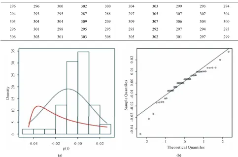
In Figure 2(a), we present the histogram of the returns ρ(.) time series (given in Table 2) while in Figure 2(b) we have the Gaussian probability plot for the same data. From these figures, one observes that the Gaussian dis-tribution does not fit well the data.

Assuming a Lévy distribution with probability density function given in (2.1) for a Bayesian analysis we con-sider the following prior distributions for δ and σ, δ ~

U(−1, −0.0271) andσ ~ U (0, 1), where U(a,b) denotes a uniform distribution on the interval (a, b). Observe that the minimum value for the ρ(.) data is given by −0.0271 and xi , that is, min



x1, , xn



 To simulate

samples for the joint posterior distribution for  and σ, using standard MCMC methods, we have used Open-BUGS software which only requires the log-likelihood function and prior distributions for model parameters. In Table 3, we present the posterior summaries of interest considering a burn-in-sample of size 5000 discarded to eliminate the initial value effect. After this burn-in-sam- ple period we simulate another 200,000 Gibbs samples taking every 10-th sample. This gives a final sample of size 20,000 to be used for finding the posterior summa- ries of interest. Convergence of the Gibbs sample algo- rithm was verified by trace-plots of the simulated Gibbs samples. From OpenBUGS output we obtain a Deviance Information Criterium (DIC) value equals to −151.7. In Figure 2, (red line), we have the plot of the fitted Lévy density with δ = −0.0487 mean and σ = 0.0391 as the scale parameter and the histogram of the ρ (.) returns.

Assuming a general stable distribution, we present in Table 4 the posterior summaries of interest obtained us-ing OpenBUGS software considerus-ing the followus-ing pri-ors: α ~ U(1, 2), β ~ U(−1, 0), δ ~ U(−0.5, 0.5) and σ ~

U(0, 0.5). In the simulation procedure, we have used a burn-in-sample of size 10,000 and another 490,000 Gibbs samples taking every 100-th sample. This gives a final sample of size 4900 to be used for finding the posterior summaries of interest.

In Figure 3, we have the trace-plots of the simulated Gibbs samples. In Figure 2, we also have the plot of the fitted stable distribution with α= 1.653, β = −0.3455, δ = 0.00782 and σ = 0.001132. We observe good fit of the table distribution (black line) The obtained DIC value is

[image:5.595.55.538.98.417.2]

Table 1. Daily price returns with n = 50.

296 296 300 302 300 304 303 299 293 294

294 293 295 287 288 297 305 307 307 304

303 304 304 309 209 309 307 306 304 300

296 301 298 295 295 293 292 297 294 293

306 303 301 303 308 305 302 301 297 299

(a) (b)

[image:5.595.53.538.462.543.2]

Figure 2. (a) Empirical return distribution; (b) Normal probability plot.

Table 2. Returns ρ(t), at time t, for n = 49.

0.0000 0.0135 0.0067 −0.0066 0.0133 −0.0033 −0.0132 −0.0201 0.0034 0.0000

−0.0034 0.0068 −0.0271 0.0035 0.0312 0.0269 0.0066 0.0000 −0.0098 −0.0033

0.0033 0.0000 0.0164 0.0000 0.0000 −0.0065 −0.0033 −0.0065 −0.0132 −0.0133

0.0169 −0.0100 −0.0101 0.0000 −0.0068 −0.0034 0.0171 −0.0101 −0.0034 0.0444

[image:5.595.62.537.572.623.2]

−0.0098 −0.0066 0.0066 0.0165 −0.0097 −0.0098 −0.0033 −0.0133 0.0067 -

Table 3. Posterior summaries for the Lévy distribution.

Parameter Mean Standard Deviation 95% Credible Interval

δ −0.04868 0.001669 (−0.05284, −0.04628)

[image:5.595.59.540.651.737.2]

σ 0.03901 0.008916 (0.02343, 0.05948)

Table 4. Posterior summaries for general stable distribution.

Parameter Mean Standard Deviation 95% Credible Interval

α 1,653 0.01639 (1.29, 1.965)

β −0.3455 0.02556 (−0.9188, −0.01257)

δ 0.00782 0.0702 (0.00549, 0.01048)

equal to −70480. From this value we conclude that the data is better fitted by the general stable distribution in contrast to the Lévy distribution (since it has smaller DIC value).

4.2. Coding and Non-Coding Regions in DNA Sequences

Crato, et al. [2] introduce the length distribution of coding and non-coding regions for all Homo Sapiens chromo-somes available from the European Bioinformatics Insti-tute. In this way they consider a transformation of the genomes in numerical sequences. As an illustration, we

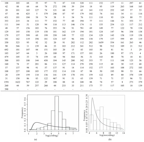
have, respectively, in Tables 5 and 6, the data for coding and non-coding length sequences for H. Sapiens chro-mosomes transformed in a logarithm scale (sequence CM000275 extracted from Table 2, in [2]).

Figure 4 presents the histograms of the data given in Tables 5 and 6, assuming a logarithm transformation. From these plots, we observe that a Gaussian distribution could not be a reasonable model for fitting the data. As-suming a Lévy distribution with probability density func-tion (2.1) for a Bayesian analysis we consider the fol-lowing prior distributions for δ ~ U (−1000, 1.0986), where 1.0986 is the minimum of the observations in

(a) (b)

(c) (d)

logarithm scale, and for σ ~ U (0, 10000). In Table 7, we have the posterior summaries of interest considering the transformed coding and non-coding data using Open- BUGS software.

Figure 4 shows the fitted Lévy density with δ = 0.9693 and σ = 3.167 (for coding data) and with δ = 4.182 and σ = 1.633 (for non-coding data). From this figure we observe that the data isnot well fitted by the Lévy distribution.

For a Bayesian analysis of the data assuming a general stable distribution, we consider the following prior dis-tributions: α ~ U(0,2), β ~ U(-1,0), δ ~ U(0,3), σ ~

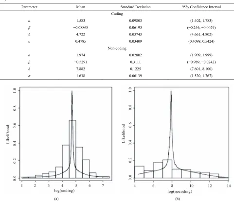
[image:7.595.54.536.251.725.2]

U(0,10). Using the OpenBUGS software, we simulated 600,000 Gibbs samples. From these 600,000 samples, we discarded the first 100,000 as a “burn-in-sample” to eliminate the initial value effects. After this “burn- in-sample” period, we took every 500-th sample, which gives a final Gibbs sample of size 1,000 to be used for Monte Carlo of the interested random quantities. Con-vergence of the Gibbs sampling algorithm was verified from trace plots of the simulated samples for each pa-rameter. Table 8 presents the posterior summaries of interest. Figure 5 shows the fitted stable distributions for coding and non-coding data. We observe good fit of

Table 5. Coding sequence CM000275.

108 103 68 55 97 73 87 110 320 111 152 177 11 297 61

42 88 68 64 78 272 190 39 254 18 95 119 263 168 165

20 101 165 127 74 121 60 97 63 141 132 252 145 57 53 47 44 425 5 379 246 87 97 179 102 74 161 34 11 116 431 101 104 58 74 38 9 54 76 111 110 95 124 80 77 353 215 34 111 77 152 77 60 394 77 111 144 51 353 77 111 144 51 128 94 110 113 146 174 11 155 254 121 117 212

48 57 156 183 76 353 54 91 781 69 149 77 122 70 134

129 145 158 119 158 181 162 119 194 181 124 147 96 358 138 179 137 599 69 199 350 149 77 122 134 129 145 158 119 158 181 162 119 194 181 124 147 96 358 138 179 137 599 69 119 350 323 95 92 32 20 91 282 112 282 1659 554 161 263 46

90 346 11 139 46 33 183 212 341 512 98 512 109 21 512

692 101 107 84 151 185 20 15 83 103 50 81 91 5 29

103 147 64 3 26 180 97 171 157 101 26 180 97 171 4 479 105 33 74 159 64 94 364 56 31 143 88 78 18 81

300 103 108 144 458 104 145 200 342 353 77 111 148 125 56

160 74 37 201 86 131 127 114 278 258 115 68 30 115 68

57 137 98 91 57 137 91 18 114 152 177 103 108 272 103

108 227 108 103 177 152 114 110 87 98 50 195 90 53 66

28 139 159 118 136 141 139 178 191 159 122 89 80 370 159

31 150 86 83 122 467 91 51 63 139 71 71 37 96 72

1591 1622 767 122 29 188 88 18 248 88 74 57 8 273 379

260 44 59 257 260 44 233 33 211 173 77 117 105 18 139 390 - - - - - - - - -

(a) (b)

[image:8.595.60.539.99.590.2]

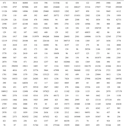
Table 6. Non-coding sequence CM000275.

473 3014 46804 1610 596 315546 82 438 122 1995 1886 2686

1 2 3 2

1490

1783 1518 2502 1230

3312 5216 1905 4273

4426 3091 2781 1494

7079 1556 2507

129 102 6083

5 8 3 2 1 1 2

1211 3807

3 1

3778 124 2610 419 1045 4157 123

1018 1486 2385

1 1

1981 1316 1143 1041 4123 2814

3377 1071

1781 1379 2766 1351

1 2 3

6403

1046 15536

1 1 1 1

1662

1193 3901 2995 1571

2 4

4831 5710 2334 1254

1041 9495

2373 3824 1836 256

2751 2060 2855 693 5216

17891 4797 507006 439 3003 254680 132 08227 3316 27057 77385 99389

11126 1 14946 21801 29460 182825 1282 2657 850 318 5045 6112

2730 110 699 392 6047 20772 7 31 270 1959

99 126 0 478 6 94 689 2308 942 1034 936 1

2590 2357 42188 686 1250 6 398 808 2001

8 129 607 3731 39 98 129 358 129 29 99 608

129 102 107 1682 608 107 5 402 86 858

2556 1917 3300 15979 94268 8404 0693 2501 149896 5176 2545 7795

9 27552 28108 441 226144 310 15 1146 1305 247 1656 3778

124 2610 419 116 10458 96 4157 123 275 84 116 4880

567 438 452 173 188 284 154 96 8536 146 1305 2073

116 8 96 275 84 116

4880 567 438 452 173 188 284 154 96 75

2074 7530 471 2014 1257 863 02886 426 369 5266 496 103

6531 398292 1 3485 547 52053 13 70 6 41846

560 4016 479 6 5064 67998 441 386840 1522 56 3721 2899

3500 23 1931 392 699 110 25884 3013 1236

7424 10533 1265 24203 3013 1236 7424 1955 7994 142294 6042 49782

290 164 8 152 117 2263 8885 409 83 489 882 2368

836 451 4275 39510 2967 1082 878 610 129 100

00912 1610 12498 4740 97823 433 1102 1320 1133 654 2979 57170

9491 2576 11103 8314 2576 60172 219 111 949 219 1158

53 1466 2036 1925 2995 423 423 13114 34 454

2709 1936 2008 870 83 425 19373 45480 1308 11169 16584 3630

7 5045 9466 67 3 13912 198 651 6242 617 985

2978 122 1039 2194 2636 1138 2212 1 1 561 437 90

1401 32 2382 167632 421 1622 145848 1639 7 90

421 1031 256 421 1357 297 66358 271 78 87 924 139

78 87 233 51764 138 66 19259 6 189

able 7. Posterior summaries, in the case of the Lévy distribution, for coding and non-coding regions of CM000275 sequence.

Parameter Mean Standard Deviation 95% Credible Interval

T

Coding

δ 0.9693 0.0260 (0.9106, 1.0160)

Non-coding

δ 4.182 0.0325 (4.114, 4.239)

σ 3.1670 0.2437 (2.7060, 3.6490)

[image:8.595.58.538.619.731.2]

[image:9.595.57.538.105.519.2]

Table 8. Posterior summaries, in the case eral stable distributi coding and non-coding regions of CM000275

Parameter Mean Standard Deviation 95% Confidence Interval

of gen ons, for sequence.

Coding

α 1.583 0.09803 (1.402, 1.783)

− (− )

(

Non-coding

α 1.974 0.02802 (1.909, 1.999)

− (− )

β 0.08868 0.06195 0.246, −0.0029

δ 4.722 0.03743 (4.661, 4.802)

σ 0.4785 0.03409 0.4098, 0.5424)

β 0.5291 0.3111 0.989, −0.0242

δ 7.882 0.1225 (7.601, 8.100)

σ 1.638 0.06139 (1.520, 1.767)

[image:9.595.60.539.109.514.2]

(a) (b)

Figure 5. ibution.

e stable distributions in

could be a good alterna-

key to obtain a go

Histograms for log(coding) and log(non-coding) and fitted stable distr

both cases. techniques (see, for instance, [11]) is the th

od performance for the MCMC simulation method for applications using stable distributions. Observe that MCMC methods are a class of algorithms for sampling from probability distributions based on constructing a Markov Chain that has the desired distribution as its equilibrium distribution. The state of the chain after a large number of steps is then used as a sample of the de- sired distribution. The quality of the sample improves as a function of the number of steps. The obtained simula- tion results for the applications in Section 4, could be easily replicated using the same auxiliary random vari- able Y defined in Section 1 and the non-informative prior distributions defined in Section 3 for the parameters of the model. More accurate posterior summaries results could be obtained using informative prior distributions

5. Concluding Remarks

The use of stable distributions

tive for many applications in data analysis, since this model has a great flexibility for fitting the data. With the use of Bayesian methods and MCMC simulation meth- ods it is possible to get inferences for the model despite the nonexistence of an analytical form for the density function. It is important to point out that the computa- tional work in the sample simulations for the joint poste- rior distribution of interest can be greatly simplified us- ing standard free softwares like the OpenBUGS software.

for the parameters of the model based on prior opinion of experts rather than using non-informative priors as it was assumed in this paper. Observe that although the non-existence of an analytical form for the density function for stable distributions, the moments could be obtained from the characteristic function defined in (1.1).

We emphasize that the use of OpenBUGS software does not require large computational time to get the pos-terior summaries of interest, even when the simulation of a large number of Gibbs samples are needed for the algo- rit

e e Processos Estocásticos- . Mazucheli gratefully ack-

. Buckle, “Bayesian Inference for Stable Distribu- tions,” Journal of the American Statistical Association Vol. 90, No. 430

doi:10.1080/01

hm convergence. These results could be of great inter- est for researchers and practitioners, when dealing with non Gaussian data, as in the applications presented here.

6. Acknowledgements

S.R.C. Lopes research was partially supported by CNPq- Brazil, by CAPES-Brazil, by INCT em Matemática and also by Pronex Probabilidad

E-26/170.008/2008-APQ1. J

nowledges the financial support from the Conselho Na- cional de Desenvolvimento Científico e Tecnológico (CNPq).

REFERENCES

[1] D. J

, , 1995, pp. 605-613.

621459.1995.10476553

[2] N. Crato, R. R. Linhares and S. R. C. Lopes, “α-stable Laws for Noncoding Regions in DNA Sequences,” Jour- nal of Applied Statistics, Vol. 38, No. 2, 2011, pp. 267- 271. doi:10.1080/02664760903406447

[3] P. Lévy, “Théorie des Erreurs la loi de Gauss et les lois exceptionelles”, Bulletin de la Société Mathématique de France, Vol. 52, No. 1, 1924, pp. 49-85.

[4] E. Lukacs, “Characteristic Functions,” Hafner Publis

häuser, Boston, 2009.

ariables,”

Ad-ical Statistics, Ed.,

i ee Primeneniya,

o. 6, 1976, pp.1006-1008.

hing, New York, 1970.

[5] J. P. Nolan, “Stable Distributions—Models for Heavy

Tailed Data,” Birk

[6] B. V. Gnedenko and A. N. Kolmogorov, “Limit Distribu-tions for Sums of Independent Random V

dison-Wesley, Massachusetts, 1968.

[7] A. V. Skorohod, “On a Theorem Concerning Stable Dis-tributions,” In: Institute of Mathemat

Selected Translations in Mathematical Statistics and Probability, Vol. 1, 1961, pp.169-170.

[8] I. A. Ibragimov and K. E. Černin, “On the Unimodality of Stable Laws,” Teoriya Veroyatnostei

Vol. 4, 1959, pp. 453-456.

[9] M. Kanter, “On the Unimodality of Stable Densities,” An- nals of Probability, Vol. 4, N

doi:10.1214/aop/1176995944

[10] W. Feller, “An Introduction to Probability Theory and Its Applications,” Vol. II. John Wiley, New York, 1971.

by [11] P. Damien, J. Wakefield and S. Walker, “Gibbs Sampling

for Bayesian Non-Conjugate and Hierarchical Models Using Auxiliary Variables,” Journal of the Royal Statis- tical Society, Series B, Vol. 61, No. 2, 1999, pp. 331-344. doi:10.1111/1467-9868.00179

[12] M. A. Tanner and W. H. Wong, “The Calculation of Pos- terior Distributions by Data Augmen-Tation,” Journal of American Statistical Association, Vol. 82, No. 398, 1987, pp. 528-550. doi:10.1080/01621459.1987.10478458 [13] M. Abramowitz and I. A. Stegun, “Handbook of Mathe-

matical Functions with Formulas, Graphs, and Mathe-

orithm,” The American Statistician,

, New York, 2004. matical Tables,” National Bureau of Standards Applied Mathematics Series, Vol. 65, Dover Publications, Wash-ington DC, 1964.

[14] S. Chib and E. Greenberger, “Understanding the Metro- polis-Hastings Alg

Vol. 49, No. 4, 1995, pp. 327-335.

[15] C. P. Robert and G. Casella, “Monte Carlo Statistical Me- thods,” 2nd Edition, Springer-Verlag

doi:10.1007/978-1-4757-4145-2