Analytical Solutions and Computer Simulations of the
Evolution of Flat Temperature Profiles in Spherical
FRRPP Systems
Gerard T. Caneba1, Mathkar A. Alharthi1,2
1Department of Chemical Engineering, Michigan Technological University, Houghton, USA 2Najran University, Najran, Saudi Arabia
Email: [email protected], [email protected]
Received April 8, 2013; revised May 27, 2013; accepted June 14, 2013
Copyright © 2013 Gerard T. Caneba, Mathkar A. Alharthi. This is an open access article distributed under the Creative Commons Attribution License, which permits unrestricted use, distribution, and reproduction in any medium, provided the original work is properly cited.
ABSTRACT
The free-radical retrograde-precipitation (FRRPP) process was recently brought into the quantitative areas of work, based on the discovery of possibility of flat temperature profiles in spherical reactive domain systems. With an ap-proximate decoupling analysis of the energy equation from the component-balance equations, these flat temperature profiles were found to be either stable or unstable. Moreover, resulting evolution of the flat profiles has been found to be expressed analytically through the so-called exponential Integral function, which has been shown to be quantitatively inaccurate during the early times of the process. This work tries to resolve this inaccuracy problem, by comparing the exponential integral results with polynomial approximation and numerical results. The result is that for the stable sys-tem, the linearized treatment of the evolution of flat temperature profiles is valid at the early 30% - 40% in the tem-perature axis, while the remainder of the evolution curve is well-represented by the application of the exponential inte-gral function. For the unstable system, the only thing that can be generalized is that both linear and cubic polynomial approximations are reasonably accurate at very small times and temperatures close to initial values.
Keywords: Flat Temperature Profile; FRRPP; Polymerization; Nonisothermal Reaction; Spherical Reactive Domains;
Exponential Integral Function
1. Introduction
A reactive spherical chain-polymerization particulate sys- tem with an exothermic heat of reaction is normally ex- pected to exhibit a parabolic temperature profile, as de- picted in Figure 1. In these systems, the idea of a flat
temperature profile is almost unheard of, and potentially beneficial in terms of operational and product uniformity. Also, the analysis of the model equations can become less complicated for these types of systems, because a field dynamics problem can be reduced to the relative simplicity of a lumped-parameter system.
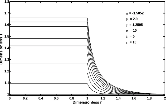
In recent publications [1,2], it has been conceptually shown that the so-called free-radical retrograde-precipi- tation polymerization (FRRPP) process can result in flat temperature profiles through a combination of thermo-dynamic, transport, and reaction-kinetic parameters in the system. This is shown in Figure 2, wherein the
pro-file starts at a uniform Dimensionless T (or θ in Equation
(6)) of 1.0. The temperature profile ends at a steady-state value of Dimensionless T = 1.83 [3]. Note that the di- mensionless r in the horizontal axis of Figure 2 is the
same as in Equation (7). This means that the reactive fluid will have ranging from 0 to 1 only. Values of
between 1 and 2 are rescaled so that they correspond to those of the stagnant fluid boundary layer.
The prediction of the possibility of the occurrence of flat temperature profiles from FRRPP systems has been advanced from a pseudo-steady-state analysis of the en-ergy balance of a model spherical reacting system un-dergoing polymerization-induced phase separation [1]. The dimensionless differential energy balance has been shown as
2 2
1 d d
Φ 0
d d
(1)
[image:2.595.147.452.75.318.2]
Figure 1. The model used for the analysis of the effect of exotherm when chain polymerization occur within a spherical par-s ticulate system that is immersed in a fluid bath. The uniform fluid bath temperature is Tb and the particulate surface
tem-perature is Ts.
0 0.2 0.4 0.6 0.8 1 1.2 1.4 1.6 1.8 2
1 1.1 1.2 1.3 1.4 1.5 1.6 1.7 1.8
Dimensionless r
D
im
e
ns
ionl
e
s
s
T
= -1.5852 = 2.9 = 1.2595 = 10 = 0 = 10
Figure 2. Temperature profile of a chain polymerization FRRPP spherical particulate system along the radial axis, = r/ro,
and with dimensionless time ( in Equation (15)) from 0 to 2.5 stepping up by 0.25. At dimensionless time of 0, the profile starts at a uniform dimensionless T (same as θ in Equation (6)) of 1.0. The temperature profile in the reaction zone (dimen-sionless r = 0 to 1) ends at a steady state value of dimensionless T = 1.83 [Alharthi, 2010]. For reference, κ is the ratio of the fluid stagnant film thickness to the particulate radius, δ is the thermal conductivity ratio of the fluid to that of the reactive particulate, and ε is the thermal diffusivity ratio of the fluid to that of the reactive particulate.
exp
(2)
The dimensionless parameters are related to the fol-lowing dimensional quantities in the energy balance and phase equilibria equations:
22
o r H
r A
o P k ao
k k
(3)
22
o P
o
s s
r H k
r B
kT kT
[image:2.595.124.473.367.586.2]a
s E RT
(5)
s T T
(6)
o r r
(7)
Δ P
oA H k a (8)
Δ P
oB H kb (9)
The phase behavior for th approximated by the linear rep
actions of the monomer and polymer (or just
polymer if the monomer conc
in Equa-tio
e polymer-rich phase was resentation
p
X aT b (10)
where XP is the product of the weight fr
the weight fraction of the entration is the same for both polymer-rich and polymer-lean phases at equilib-rium, as the case for the PS-S-Ether system [4,5]. Since Equation (10) provides a mesoscopic-macroscopic rela-tionship between the temperature and monomer compo-sition, it allows the decoupling of the mesocopic-mac- roscopic analysis of the time evolution behavior of the thermal aspect of the system from compositional aspects, until the details of the kinetics of microphase separation behavior is incorporated in the field equations.
In order to quantitatively characterize the relatively lower inefficiency of radical maintenance in free-radical polymerization systems, the expression for XP
n (10) can be modified to include a polymer radical efficiency factor fP; thus,
P p
p p M p
X f X X (11)
Also, a and b in Equation (10) were proposed to be obtained from experimental data poi
ria experiments. It should be note ra
Φo and Equation (2) became
nts of phase equilib-d that the polymer dical efficiency factor, fP, is related to the initiator effi-ciency, f, in free-radical polymerizations in a relative sense, i.e., for the same monomer, solvent, their concen-trations, and operating temperatures, fP is relatively high when an initiator with a relatively high f is used. The reason is that initiation is the starting point in time when inefficiencies of radical production take place. The sur-vival of propagated radicals will later depend on the ef-fectiveness of the FRRPP radical trapping mechanism, which should result in fP < f. For example, in FRRPP of polystyrene-styrene-ether systems using azobis diisobu-tylonitrile (AIBN) as initiator, fP was found to be in the order of 0.20 [1,4] even though f was known to be around 0.57 [6].
For the expectation of a flat temperature profile, θ= 1 for η= 0; thus, the dimensionless source term was
sym-bolized as
exp
o
(12) Then, a combined dimensionless quantity was intro-duced to quantitatively characterize str
ior, wherein the reactive polymer-rich fla
ict FRRPP domains attained t temperature profiles. The dimensionless quantity was symbolized by Cn (pronounced see-enye), and defined as
11 1 exp
Cn
o
Values of from computational efforts indicated that for th process, it should be a
−1000 for a flat temperature profile [1].
ditional criteria fo
one, because the value of α automatically becomes a
st
(13)
n C
e FRRPP t least below
In the unsteady-state analysis of the FRRPP system, the occurrence of the flat temperature profile from FRRPP systems was reinforced, with ad
r stability of steady-state behavior [2]. For a stable steady-state system, it was found that the quantity α < 0 even for an insulated reactive domain system. For > 0, the reactive system was found to be under control with the possibility of a flat temperature profile through rela-tively ineffective heat removal from the fluid. With more aggressive heat removal from the fluid, the temperature profile in the reactive solid becomes more of a parabolic one.
When the monomer concentration drops to low enough values, the reactive system automatically reverts to a stable
negative number [1]. This happens either locally (due to relatively fast reaction rate compared to diffusion rate, or polymer domain densification [2]) or in the overall reactive system, due to depletion of monomer molecules.
With assumption of a flat temperature profile, the field energy balance equation was simplified to a mixing-cup ordinary differential equation and later analyzed for its ability characteristics [2]. Results from the field partial differential equation correspond to the reacting sphere with insulated surfaces. An analytical expression for the modified dimensionless temperature () vs dimension- less time (τ) was also obtained for the flat temperature profile reactive spherical domain with insulated bound- ary surfaces as
1
1
e Ei Ei
Θ Θ
(14)
in which the dimensionless time was expressed as
2
s
o t r
and the modified dimensionless temperature (), and are obtained as
Θ s b T T
(16)
s
b T T
(17)
s
b T T
(18) Note that Tb is the bulk fluid temperature while Ts is the reactive particle surface temperature (Figure 1).
The function, Ei or the Expo
[7], is a special transcendental function which has been fo
nential Integral Function
und to occur in only a few experimental systems; thus,
t exp t
d
Ei x t
t
(19)It can be evaluated through the following infinite se-ries expansion for real positive arguments (x > 0):
1 Euler Mascheroni Constant ln
! k k Ei x x x k k
(20)
The Euler-Mascheroni constant (also called Euler’s constant) has been cited to be equal to 0.577215664 should be noted from Equation (20) that the Ei fun approaches −∞ at its argument (x) approaching zero from th
p-pr
ted for the as-ometry
ameter an dimensional form the lumped- 9... It ction
e positive side (0+). This is reflected in inaccuracies in results from direct evaluation Equation (14) at τ→ 0+.
In this paper, inaccuracies of the analytical evaluation of Equation (14) are addressed, by comparing predictions of the evolution of flat temperature profiles in FRRPP systems from numerical solutions and analytical a
oaches. Numerical solutions used include the evalua-tion of the field energy equaevalua-tion and its lumped-param- eter version for a flat temperature profile. Analytical me- thods employed here include the use of the exponential integral function (Equation (14)), as well the Taylor- Series-based polynomial approximations.
2. Generalized Mathematical Model of
FRRPP Domains
Since the diffusive term could be neglec sumption of a flat temperature profile, then the ge of the system does not matter and a lumped-par
alysis can be made. In
parameter energy balance around a reactive particle can be more conveniently expressed using the convective heat transfer coefficient, h, as
dˆ d
S PS b
T
C q hA T T
t
(21)
where A is the heat transfer area. For insulating boundary surfaces, h = 0, and thus
dΘ
Φ Θ e
d
Θ (22)
Thus, the integral operation for the determination of τ
at any value of is
Θ Θ e dΘ
(23)sed as the starting material for poly-nomial approximation at relatively small values of di-mensionless time, τ, wherein the app
with the integrand.
etailed field simulation results were also obtained. The following conditions have been
de-1 Θ Equation (23) is u
roximation is done
3. Computer Simulation Results of IVP-PDE
In order to validate results of polynomial approximations of Equation (23), d
duced for the occurrence of a flat temperature profile in FRRPP systems:
1) Cn 1000, α < 0, 0, 0, and h > 0 2) Cn 1000, α < 0, 0, 0, and h = 0 3) Cn 1000, α > 0, 0, 0, and h = 0 Note that only Conditions 2 and 3 are covered in this paper.
4.
lynomial
xima
ns from
ction F() correspond to the integrand of Equation (23); thus,
Po
Appro
tio
Ea
rly-Time
s Behav
ior
Let the fun
Θ e Θ F Θ Application of the
(24)
Taylor series expansion at the initial dimensionless time of zero and dimensionless tempera-ture = 1 leads to
1 2 2 1 1 d 1 d F F F 2 1 3 3 3 1 d 1 2 d1 d 1
3! d F F (25)
The software Mathematica® is used to deriv
ous derivatives in Equation (25), and the following re-sults were obtained up to the cubic derivative.
e the
vari-
2 2
d e e
d
F
(26)
2 2 2
2 3 4 3
2 2
d 2 e e 2 e
d 2 e F (27)
3 3 2 3
3 4 2 3 6
2 2
5 4 2
4 3 2
d 6 e 6 e e
d
6 e 3 e
6 e 6 e
F (28)
In order to understand the F() function, it is plotted in Figure 3 at typical parameter values for both stable
and unstable systems, wherein the flat temperature pro-file is proposed to occur.
From this figure, the area under the curve can be ob-ta
resulting plots of the Dimen-si
r. This exercise is very important for va
ined to be equal to the dimensionless time, . Note that for the stable system, the value of approaches infinity at the steady-state value of 5. With the two sets of pa-rameters in Figure 3, the
onless temperature, , vs Dimensionless time, , is shown in Figure 4.
Since the use of the Exponential Integral function, Ei, as defined in Equation (19), is not well understood in FRRPP systems, comparisons with straight numerical solution and Taylor Series approximations are made and reported in this pape
lidation of a new conceptual phenomenon that is ex-pressible with a rarely used transcendental function.
0 2 4 6 8 10 12 14 16 18 20
1 2 3 4 5
F( ) -0.1,0.5,1 4,-2.5,1
Figure 3. Plots of F() vs from Equation (24) for typical sets of parameters representing stable and unstable systems. The legend indicates the triplet of parameters
, ,
,parameters wherein the stable system represents the set of
with negative .
vs for Flat Temperature Profiles
4 5 6 0 1 2 3
0 4 8 12 16 20
-0.1,0.5,1
4,-2.5,1
Figure 4. Evolution of flat temperature profile from typical parameter sets for stable and unstable systems. The legend indicates the triplet of parameters
, ,
arameters
, wherein the stable system represents the set of p with negative . Also, note that as increases beyond 20, the value of
s,
ure
een
% -range, while th
asymptotically approaches the steady-state value of 5.
5. Results of Polynomial Approximations
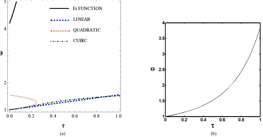
Figures 5(a) and 6(a) show polynomial approximation
results of vs for flat temperature profile histories involving typical stable and unstable parameter system which could be compared to numerical results in Fig 4. This stable system curve in Figure 4, in turn, has b
found to compare very well with Figure 5(b), which is
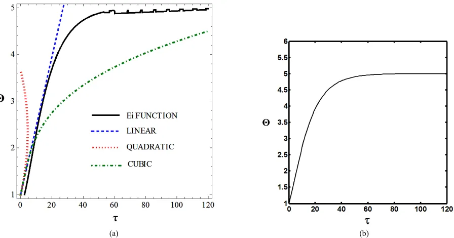
the numerical result of the solution of the full differential equation in Equation (22). For a representative unstable system, the dashed-curve result in Figure 4 is compared
with polynomial approximation results in Figure 6(a).
This representative unstable system curve in Figure 4, in
turn, has been found to compare well with Figure 6(b),
which is the numerical result of the solution of the full differential equation in Equation (22). In addition, expo-nential integral results are shown for given parameter sets in Figures 5(a) and 6(a). Figures 7(a) and 7(b)
show expanded abscissa scales for Figures 5(a) and 5(b),
for additional comparisons. On the other hand, Figures 8(a) and 8(b) show shorter time behavior for conditions
associated with Figures 6(a) and 6(b).
These plots indicate the validity of the use of the nu-merical approaches, compared to the Ei approximation method using Equation (14). If one uses the polynomial approximation, for < 0, the linear approximation would be quite accurate in the initial 60% - 70
(a) (b)
Figure 5. (a) Approximation results of vs for flat temperatu istories involving a typical stable parameter s stem, represented by
re profile h y
0.1, parameter
0.5, system, re
1.0; (b) Numerical s for flat temperature profile histories involving presented by
results of v 0.1, 0.5, 1.0. a typical stable
(a) (b)
Figure 6. (a) Approximation results of vs for flat temperat e histories involving a typical stable parameter system, represented by
ure profil 4.0,
table param 2.5, eter system,
1.0; (b) Numeric vs for flat temperature profile histories involving a typical uns
al results of
represented by 4.0, 2.5, 1.0.
6. Conclusio
n
linear Taylor series approximation up to 30% - 40% ofhe quantitative analysis of the occurrence of the flat in spherical FRRPP systems indicates
hes to predict its evolution would
the -range, and continuing to steady-state condition with the use of the Exponential Integral, Ei, function. For T
temperature profile that numerical approac
be reasonably accurate. If an analytical approximation is to be done, for < 0, the approach would be to use the
> 0, the only conclusion that can be made is that both linear and cubic polynomial approximations are reasona-bly accurate at very small times and low -values, i.e., at
[image:6.595.81.517.82.314.2] [image:6.595.86.516.374.598.2]
(a) (b)
Figure 7. (a) Longer abscissa range version of Figure 5(a), for flat temperature profile histories involving a typical stable pa-rameter system, represented by 0.1, 0.5, 1.0; (b) Longer abscissa range version of Figure 5(b), for flat temperature profile histories involving a typical stable parameter system, represented by 4.0, 2.5, 1.0.
(a) (b)
Figure 8. (a) Shorter abscissa range version of Figure 6(a), represented by 4.0, 2.5, 1.0; (b) Shorter ab-scissa range version of Figure 6(b), represented by 4.0, 2.5, 1.0.
ichiga entally Benign Functional
Scholarship Program,
Na-e FRR ocess.
7. Acknowledgements
he authors are grateful for the support of the M n
tigation of th PP pr T
Tech Center for Environm Materials, the King Abdullah
jran and Michigan Tech Universities that allowed the continued work and publication of the quantitative inves-
REFERENCES
[image:7.595.76.524.86.321.2] [image:7.595.69.529.380.613.2]2010.
[2] G. T. Caneba and Y. L. Dar, “Emulsion Free-Radical Re-trograde-Preci ” Springer-Verlag, Heidelberg, 20 42-19872-4
pitation Polymerization, 11. doi:10.1007/978-3-6
University, Houghton, 2010.
[3] M. A. A. Alharthi, “Dynamic Thermal Behavior of the Free- Radical Retrograde-Precipitation Polymerization (FRRPP) and Related Processes,” M.S. Thesis, Michigan Techno- logical
[4] Y. Dar and G. T. Caneba, “Transport Phenomena Aspects of the Free-Radical Retrograde-Precipitation Polymeriza- tion (FRRPP) Process,” Chemical Engineering Commu- nications, Vol. 189, No. 5, 2002, pp. 571-607.
doi:10.1080/00986440211745
[5] B. Wang, Y. Dar, L. Shi and G. T. Caneba, “Polymeriza- tion Control Through the Free-Radical Retro
cipitation Polymerization (FRR
grade-Pre- PP) Process,” Journal of Applied Polymer Science, Vol. 71, No. 5, 1999, pp. 761- 774.
doi:10.1002/(SICI)1097-4628(19990131)71:5<761::AID-APP10>3.0.CO;2-S
[6] G. Odian, “Principles of Polymerization,” John Wiley and Sons, New York, 1991.
.1. Alphabets
n (8), dimensionless quation (9), dimensionless nergy for reaction, J/mol
ation (24)
1.
k: Thermal conductivity of the reaction fluid , m or cm
1.
quation (11) lymer in Equation (11)
xponential rate coefficient
(Equa-tio Source
Te
1.
ls
β: Dimensionless version of b from Equation (4)
γ: Dimensionless activation energy, defined in Equa-tion (5)
η: Dimensionless radius, defined in Equation (7)
mensionless temperature, defined in Equation (1
d in Equation (15)
Eq
1.5
ntial integral function, defined in
Equa-P
ΔH
ns (3),(4),(8),(9)
t, Li/mol-s
m at the center of th
m
[7] J. Spanier and K. B. Oldham, “An Atlas of Functions,” Hemisphere Publishing Corporation, New York, 1987.
1. Nomenclatures
1
1.1.1. Upper Case
A: Defined in Equatio
B: Defined in E
E: Activation e
F: Defined in Equ
R:Universal gas constant,J/mol-K
T: Absolute temperature, K
X: Defined in Equations (10)-(11), dimensionless
1.2. Lower Case
a: Defined in Equation (10)
b: Defined in Equation (10)
r: Radial distance
2. Subscripts
a: pertains to Activation ene
M: Pertains to monomer in E
rgy (Equation (5))
P: pertains to po 0: pertains to Pre-e
ns (3),(4),(8),(9)) or Dimensionless Energy rm ( Equation (12))
3. Superscripts
P: Pertains to polymer-rich phase in Equation (11)
1.4. Greek Symbo
α:Dimensionless version of a from Equation (3)
ρ: Density, g/cm3 or kg/m3
θ:Dimensionless temperature, defined in Equation (6)
: Di 6)
: Dimensionless time, define
Φ: Dimensionless heat of polymerization, defined in uation (2)
. Other Symbols
n
C : Defined in Equation (12), dimensionless
Ei(x): Expone tion (20)
f : Polymer radical fraction
P
ko’: Pre-exponential factor of rate coefficient, defined in Equatio
: Heat of polymerization, J/mol
kP: Propagation rate coefficien
Φ0: Dimensionless energy source ter e particle, defined in Equation (12)
r0: Particle radius, cm or
XP: Defined in Equation (11)
P M
X : Defined in Equation (11)
P P