An Example of an Investment Model That Makes Something Out of Nothing (Sort of): Implications for Building Applied Mathematical Models

(1)

An Example of an Investment Model That Makes

Something Out of Nothing (Sort of): Implications for

Building Applied Mathematical Models

Greg Samsa

Department of Biostatistics and Bioinformatics, Duke University, Durham, USA Email: [email protected]

Received April 13, 2013; revised May 13, 2013; accepted May 20, 2013

Copyright © 2013 Greg Samsa. This is an open access article distributed under the Creative Commons Attribution License, which permits unrestricted use, distribution, and reproduction in any medium, provided the original work is properly cited.

ABSTRACT

Two related and under-studied components of modeling are: a) the process by which simplifying assumptions are derived; and b) the process by which tests of model validity are designed. This case study illustrates these processes for two simple investment models: a) a version of the model supporting classical portfolio theory; and b) a version of a mean-reverting model consistent with some of the tenets of behavioral finance. We perform a simulation that demonstrates that the traditional method of empirically assessing the performance of value investment strategies is under- powered. Indeed, the simulation illustrates in a narrow technical sense how to make something out of nothing; namely, how to generate increased returns while reducing risk. Analyzing the mechanism underpinning this counter-intuitive result helps to illustrate the close and sometimes unexpected relationship between the substantial assumptions made about the systems being modeled, the mathematical assumptions used to build models of those systems, and the structure of the experiments used to assess the performance of those models.

Keywords: Mathematical Modeling; Financial Modeling; Sociology of Science

1. Introduction

1.1. The Model Development Process

The development of applied mathematical models takes place within a framework that is simple, elegant, and sometimes under-appreciated [1]. To summarize this process:

Step 1: Make simplifying assumptions about the system being modeled. The modeler acknowledges at the start of the process that these assumptions will not be fully realistic, but instead are intended to reflect the most important features of the system being studied.

Step 2: Develop a model around those simplifying assumptions.

Step 3: Collect data and assess the fit of the model to the data. Ideally, this assessment will involve multiple datasets, collected under diverse circumstances. Explore a) where the model fits the data well; and b) where the model fits the data poorly. If the model fits enough of the data sufficiently well then it is tentatively accepted and conclusions about the system being studied are drawn. If not, focus on the discrepancies (e.g., in which experi-

ments did the model fail?) revise the model assumptions —typically, in the direction of an incrementally more complex description of the system being studied—and begin step 3 again.

1.2. What Makes a Good Model?

A “good” model typically is parsimonious, yet fits the data sufficiently well. Moreover, it captures the most important features of the system under study. It is this combination of both empirical and theoretical evidence that gives the modeler confidence that the model might generalize to new data sets.

1.3. What Can Go Wrong?

(2)

tant. This danger is particularly acute when the modeler is a mathematician or statistician without deep expertise in the system under study and the substantive experts are unfamiliar with the nuances of the modeling.

Another danger in modeling is that the experiments used to test the model aren’t sufficiently rigorous. To use a medical example, one component of personalized medicine is the development of predictive models—for example, a logistic regression model that predicts the prob- ability of a patient having a serious complication from chemotherapy. If this model is originally developed using patients from tertiary care medical centers and all of the validation studies are performed using similar patients, it would be reasonable for a user to be concerned that the model might not perform as well when applied to patients receiving care in less specialized facilities.

2. Example

We provide an example of how making a seemingly trivial modification to a simple economic model and then performing the evaluation of that model using the current state of the economic science provides surprising results —so surprising, indeed, that they appear to violate one of the most basic tenets of investment theory and thus appear to “make something out of nothing”.

2.1. Conceptual Framework

The conceptual framework for the example is the simple errors in variable model under which classical portfolio theory is derived. In this model, the returns for an investment are assumed to be derived from independent random samples from the same statistical distribution. For example, the annual returns for an index fund that tracks the overall stock market might be modeled as a sequence of independently generated Gaussian variables, with mean 0.10 and standard deviation 0.15.

Economist don’t always assume that the distribution of investment returns is Gaussian—for example, these returns are often assigned log-normal, Levy or other types of distributions. For the purposes of understanding the model development process, what is much more important is not the shape of the distribution of returns but rather the fact that the returns from year to year are assumed to be independent. In fact, the average return isn’t central to the present argument. Accordingly, we can assume that the price of the investment at any point in time, denoted by Yi, is:

1

i i Y Y_ E_i.

Here, the Ei are independently, identically distributed Gaussian random variables with mean 0 and standard deviation σE. Under this highly simplified model, stock prices will follow a random walk.

The link between the features of the system presumed to be most important and the model is provided by Ei. Specifically, if it is assumed that the stock market is a “perfect market” with large numbers of well-informed investors, none of whom are large enough to affect prices, then it follows that the current stock price Yi represents all available information. (Otherwise, arbitrage will push the price toward a value that reflects this information.) Moreover, it follows that at the next time point stock prices will only change in response to the new information Ei+1. This new information—for example, a tsunami, a change in government policy—is unpredictable, since otherwise it would have already have been reflected by the previous Yi. Accordingly, the series of perturbations (i.e., “shocks”, “errors”) are independent. Once this errors in variables structure is assumed, the other main elements of classical portfolio theory become logical consequences [2].

The assumption that the stock market is a perfect market—and thus that the Eis are independent—illustrates steps 1 and 2 of the modeling process. Certainly, economists don’t believe that any actual market is “perfect” in the sense of the above. However, it might be plausible to posit, as a first approximation to describing an exceedingly complex system, that the stock market is perfect and then to explore how much (or little) harm is done by such an assumption.

2.2. Relationship between Risk and Return

Apart from the assumption about independence, the above model embeds within Ei a second critical feature of the system—namely the variability in stock prices as quanti- fied by σE. When σE is small, as is the case for estab- lished companies with dependable prospects, the stochastic path followed by the stock price is less variable than for more speculative enterprises (for which σE is larger).

In classical portfolio theory, volatility in prices is considered to be synonymous with risk. The rationale— which is ultimately derived from the assumption that the system being studied is a perfect market—is that all other information, including information about “business risk”, must already been accounted for in the current stock price.

(3)

returns) to re-adjust.

The conclusion that higher (expected) returns require accepting additional risk is highly intuitive and, indeed, one of the original benefits of classical portfolio theory was that it provided a mathematical justification to support this intuition.

2.3. Behavioral Finance Critique

Proponents of behavioral finance argue that changes in stock prices are predictable, at least in some cases. As an example, they argue that when a fundamentally sound company such as Johnson & Johnson (JNJ) suffers temporary reversals in the performance of its businesses investors will engage in a predictable over-reaction and sell the stock en masse. One proposed explanation for this behavior is that this selling is an evolutionarily-selected behavior—our surviving ancestors reacted to the “bad news” that the sound in the bushes might be a lion by running first and asking questions later. Another proposed explanation is that the hedge fund managers and other large speculators that set stock prices in the short run have financial incentives to engage in herding behavior. Regardless of the explanation, the selling causes the price of JNJ’s stock to become temporarily under- priced, eventually leading to a (somewhat) predictable counter-reaction whereby the returns for this stock are better than would be otherwise anticipated. The strategy of “value investing” attempts to take advantage of this putative predictability in market behavior.

Value investing is but one example of the sort of pre- dictions that are generated by the conceptual model(s) underlying behavioral finance. To modify the above model to take into account value investing requires adding complexity to its structure.

2.4. A Revised Model for “Safe Haven Companies”

The debate between supporters of modern portfolio theory and those of value investing essentially amounts to one between nihilists and fundamentalists. The assertion that all available information is contained in the current stock price is nihilistic—as it implies that for the purposes of predicting future stock prices the fundamental elements of the company (e.g., its products, its business model, its management) don’t matter. Fundamentalists argue the reverse—not only does this information matter but, although it might be ignored by the market in the short-term, truth about long-term corporate performance will eventually win out.

There is one point about which these two schools of thought agree—namely, that stocks of “safe-haven” companies such as Johnson & Johnson (JNJ) have lower risk than average. The nihilists base their opinion on the low

level of volatility in their stock prices. Fundamentalists base their opinion on the fact that these are large, well- financed companies that offer products that consumers must continually repurchase (e.g., band aids), and thus they have a lower level of “business risk” than average.

In practice, the prices of safe-haven companies evidence a stronger tendency to regress towards the mean than do most others. One explanation for this phenomenon is that, because their stream of earnings and dividends is so predictable, their “intrinsic value” can be estimated with a much higher degree of accuracy than is the case for other companies. Indeed, it can be postulated that the prices of safe haven stocks most often depart from this intrinsic value because of the view that large institutional investors have about the other stocks in the market. When these investors are feeling speculative, they sell the safe haven stocks in order to raise money to buy other companies. When these investors are stricken with panic, they do the opposite. This amounts to a tendency for historically low prices to regress toward their mean—a trend that becomes increasingly strong as the price diverges from its intrinsic value.

Accordingly, a model of the behavior of the prices of safe-haven stocks can be specified as follows:





1 1

i i i

Y Y  T Y  Ei, where α > 0 and T represents

the company’s “intrinsic value”. When the price at time i - 1 is less than intrinsic value, will exceed 0, and thus its impact will be to push the next price toward intrinsic value.



T Yi 1

  _



To comment on the process of model formulation, although the “intrinsic value” T for a safe haven company can’t be observed, it is a quantity about which most investors would roughly agree—thus, the intention is that T quantifies one of the fundamental properties of the system under study. The term α is intended to represent another such fundamental property; namely, the tendency for (some) stock prices to regress toward a (generally understood) target value. T and α represent an incre- mental increase in the complexity of the original model; moreover, when α = 0 the original model is recovered.

2.5. A Value Investment Strategy

The goal of “safe-haven value investors” is to buy safe- haven companies at prices below their intrinsic value, to hold these companies until their prices exceed their intrinsic values, and thus to obtain superior risk-adjusted returns. Nihilists deny that it is possible for any strategy to obtain superior risk-adjusted returns.

2.6. Design of an Experiment

(4)

is operationalized as follows: The value investor is seek- ing mature, fundamentally sound companies whose stock price has suffered a temporary reversal. Many mature companies pay dividends, and when the stock price falls the dividend yield (i.e., the dividend divided by the stock price) rises. Thus, stocks with (temporarily) high dividend yields should out-perform the market (after appro- priate adjustment for risk).

The steps in the algorithm to test this hypothesis are as follows:

1) Define the strategy in sufficient detail to be implemented by computer (e.g., select all stocks whose current dividend yield is at least 5%.

2) Using a database, select (and pretend to buy) all stocks with the desired characteristics as of a certain date such as 1/1/2000.

3) Hold the stocks for a specified period such as 1 year.

4) Using the same database, pretend to sell these stocks as of a certain date such as 12/31/2000.

5) Based on the difference between the purchase and sales prices (plus any dividends received), calculate a hypothetical rate of return for the time period in question.

6) Repeat the process for multiple time periods (e.g., 1/1/2001-12/31/2001, 1/1/2002-12/31/2002, etc.).

7) Using the data from all the time periods, calculate an estimated rate of return, plus a standard deviation.

8) Use this latter standard deviation as an input to risk- adjust the estimated rate of return

9) Compare the risk-adjusted return of the strategy with that of the overall market. If the strategy being tested outperforms the market the theory is supported—otherwise, not.

To date, the experiments that have tested the value investment hypothesis have all taken this form (albeit with different criteria for operationalizing the value investment strategy). The results haven’t been definitive. In general, and consistent with a broader literature on behavioral finance, such value-based strategies do tend to outperform the market, but by only a modest amount. This relative outperformance supports the positions of both parties. The fundamentalists point to the outperformance and, indeed, an entire industry has developed around the idea of behavioral-financed-based investment. The nihilists point to the modest levels of outperformance as evidence of how difficult it is to “beat the market”, and hold out the possibility that more sophisticated methods of risk-adjustment would cause the apparent outperformance to disappear altogether.

2.7. Current Critique of the Critical Experiment

It turns out that the above experiment, although easy to describe and perform, is difficult to interpret. This cri-

tique isn’t central to the present argument, and thus is relegated to Appendix 1. For now, we will stipulate that the experiment can be performed and interpreted as intended.

2.8. A New Critique of the Critical Experiment

Perusal of Appendix 1 demonstrates that the investment literature contains criticisms of every step in the above algorithm with the exception of the innocent-sounding step 3 (hold the stocks for a specified period such as a year). Apart from being intuitively natural, the original motivation for fixing the holding period was based on economic theory. Specifically, stocks are often held until a specific date—for example, an “investment horizon” might close on the date of a scheduled retirement, on the date that the investor expects to enter college, etc. Much of investment theory begins by fixing the investment horizon.

However, in actual practice investors seldom buy and sell stocks on pre-specified dates. They try to time their buying in order to obtain bargains, and they try to wait until the stocks they hold become over-valued before they sell. If they succeed in “timing the market”, their returns will exceed those of the strategy of buying and selling at pre-specified dates. Indeed, the greater the volatility in the stocks that they hold, the greater is the potential increase in returns associated with buying and selling op- portunistically, and the greater is the loss in statistical power associated with performing assessments in the usual fashion.

This inconsistency between the behavior of actual investors and the assumption that investors buy and sell at pre-specified time periods (i.e., an assumption of the test of the models, albeit not of the models themselves) turns out to have unexpected consequences.

3. Methods

3.1. A Simulation-Based Test of a Strategy for Safe Haven Stocks

To design a test of the value investment hypothesis, assume that the investor has a relatively long investment horizon such as 10 years, each of which consists of 250 trading days. On trading day 0, the investor purchases a stock at its intrinsic value of $100. The holding period is indefinite—the investor will sell the stock when its return is R. For example, if R = 4% the investor will sell the first time the stock price reaches $104. Once the stock is sold, another stock with similar characteristics is bought and the process is repeated. At the end of the investment horizon, the stock that the investor owns is sold, regardless of price.

(5)

mary assumptions held by the nihilists; namely, that investors are unable to consistently identify those situations where the price of a stock is less than its intrinsic value. Instead, what is being assumed is that investors are merely no worse than average in selecting among safe-haven companies. Accordingly, what is being tested is a strategy that is weaker than what value investors are actually attempting to accomplish.

3.2. Expected Returns for the Strategy

The intrinsic value of actual safe-haven companies is expected to increase over time, due to the compounded growth of their earnings. Here, for simplicity, we have assumed that the intrinsic value remains constant. Ac- cordingly, if the nihilists are correct the expected return of this strategy, estimated by following the returns of a hypothetical large cohort of investors each having an investment horizon of 10 years, should be 0.

On the other hand, if the observed return exceeds 0, we will have demonstrated that the returns of safe-haven companies can be enhanced by taking advantage of the stochastic nature of their prices. This enhancement will only be observed for the minority of stocks demonstrat- ing mean-reversion. Accordingly, the returns of the safe- haven companies will exceed those of some of the other companies in the market with higher levels of risk. In the limited sense defined above, this will provide a counter- example to the investment maxim that in order to obtain increased gains investors must always accept increased risk.

[image:5.595.55.288.663.736.2]

4. Results

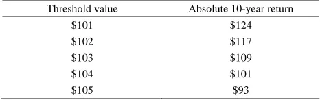
Table 1 presents results under the following scenarios. The investment is purchased at the intrinsic value of $100. The distribution of the errors is Gaussian with mean 0 and standard deviation 1. The parameter representing regression toward the mean, α, is 0.01. The investment horizon is 10 years (2500 trading days). If the price exceeds the threshold value, a profit is taken and the simulation is re-set—that is, another stock is purchased at $100. On day 2500 the stock is sold. For example, setting the threshold value to $101, on average the value of the investment at day 2500 is $224, for an absolute return of $124 (i.e., $224 minus the original $100).

Table 1. 10-year absolute returns, keeping the purchase price of $100 constant, varying the threshold value.

Threshold value Absolute 10-year return

$101 $124 $102 $117 $103 $109 $104 $101 $105 $93

For the above set of parameters, as the threshold value decreases the absolute return increases. For a threshold value of $101, the absolute return of $124 corresponds to an annualized return exceeding 8%. Please note that this $124 is an excess return—that is, an excess return above the 0% that would be expected from a buy-hold strategy, since it is assumed that the intrinsic value is unchanged over the course of the simulation.

5. Discussion

Our primary purpose here is to illustrate the impact that seemingly subtle changes in both model assumptions and testing strategy can have an impact that is both unexpected and strong. We found a surprising result—namely, that by making the natural and seemingly innocent assumption that investors hold stocks for a fixed period of time, their returns will be underestimated. This result only holds for the subset of stocks that exhibit mean reversion. However, for such stocks we have provided a counter-example to the usual relationship between risk and return. Mean-reverting stocks have less business risk than average, and also exhibit lower volatility in their prices. Nevertheless, “harvesting their volatility” can increase their returns notably—so much so that they can exceed the returns of “riskier” and “lower-quality” stocks. Moreover, this example illustrates that traditional studies of value investing strategies underestimate the returns associated with those strategies.

Our demonstration has a number of limitations. First, the model for the price behavior of mean-regressing stocks is simplistic. The model for Ei doesn’t take into account the possibility that a stock can move from a safe haven to a disaster. For example, the oil giant BP would have been a natural candidate for mean reversion, right up until the moment of the Gulf oil spill.

Second, the parameters of our model were chosen for purposes of illustration, and were not empirically estimated. In particular, if the variability of the error term E in our model is unrealistically large, so will be the impact of regression toward the mean. Our simulations are intended as a proof of concept to demonstrate than an effect is present, but not necessarily to estimate its magni- tude.

Third, since this paper is not primarily concerned with the empirical performance of actual investment strategies, we have not engaged in the traditional data-based assessment of the returns associated with the above strategy. Interested readers are encouraged to perform such a test, if desired.

(6)

medicine cabinet stocks”) evidence a strong correlation among their prices. On the other hand, such an assumption is consistent with the well-documented phenomenon of “sector rotation”—presumably, an investor could always find an out-of-favor sector of the market and then select a high-quality company within that sector under the assumptions that: a) the current stock price is proba- bly no higher than its intrinsic value; and b) because the company is of high quality, it will eventually be in sufficient demand among investors to cause the phenomenon of regression toward its mean.

Finally, when taken literally, the strategy being tested would suffer considerable slippage due to commissions and taxes. However, it is equally applicable to longer time frames. Presumably, the investor would want the time frame to be long enough to comfortably avoid over- trading, yet short enough so that there remains volatility to be harvested.

In summary, investors (as differentiated from pure speculators) all attempt to buy stocks at reasonable prices and must all cope with price volatility. Value investors hope that volatility will temporarily push the price of stocks so low that they can buy with a margin of safety (i.e., at far below their intrinsic values). Whether this can be done consistently is a subject of debate. What we have contributed to this debate is a counter-example—demon- strating that excess risk-adjusted returns are possible by using a volatility-harvesting strategy even when stocks are purchased at their intrinsic values, (so long their prices exhibit the tendency to regress toward their means). Of course, nothing in this paper constitutes actual investment advice, and the fact that we have demonstrated this counter-example (albeit under restrictive assumptions) doesn’t necessarily imply that readers should try this with their own money. But it does imply that readers should pay particularly careful attention to the substantive implications of the assumptions that are embedded within their mathematical models, and also to how those models are tested.

6. Comment

Mathematical modeling of non-deterministic phenomena —of which investment returns are but a single example— contains elements of both art and science. There is a vast literature within economics that discusses the “science” of economic modeling—for example, which distributional assumptions to apply under which circumstances. Other disciplines have similarly large literatures on how to apply the scientific aspects of modeling to their particular circumstances. Moreover, the discipline of statistics provides a unified framework for thinking about the science of modeling in the presence of uncertainty.

As a representative illustration of the statistical perspec-

tive, consider the May 16, 2013 Wikipedia entry on “statistical modeling”: “Astatisticalmodelisaformalization of relationships between variables in the form of mathe- maticalequations. Astatisticalmodeldescribeshowone or more random variables are related to one or more othervariables. Themodelisstatisticalas thevariables are notdeterministicallybutstochasticallyrelated.” For an economic application, “statistical” could be replaced with “economic” to obtain a definition that might easily appear in an economic textbook: “An economic model is a formalization of relationships between economic vari- ables in the form of mathematical equations. It describes how one or more random variables are stochastically related to one or moreothervariables.”

For the present purposes, what is particularly striking about the above definitions is their narrow perspective. Most importantly, they conceptualize modeling as for- malizing relationships among “variables” rather than among “underlying constructs”. If the variables adequately represent the underlying constructs (e.g., if volatility in stock prices is an adequate representation of investment risk), and if the mathematical equations adequately represent the most fundamental relationships between these constructs, then the “science” of statistical modeling works well. In contradistinction to the “science” of modeling, the “art” of modeling consists, among others, of determining how best to represent the underlying constructs, and how best to represent the relationships among these constructs through mathematical equations. Just as the Wikipedia definition addresses the science but not the art, the literature on modeling is similarly skewed.

One might reasonably hypothesize that the relative in- attention to the art of modeling is due to its qualitative nature. Much of the science of modeling can be described quantitatively (e.g., how closely a particular model meets an optimality criterion) and translated into actionable protocols (e.g., to determine the optimal regression coeffi- cients in a linear regression model solve the normal equations), both of which are concrete. On the other hand, while the art of statistical modeling includes some core principles (e.g., parsimony) and can be partially described by algorithms (e.g., the 3-step algorithm in Section 1.1), it cannot be reduced to a simple protocol.

In the absence of specific protocols from the literature, then, what practical advice might be provided about the more artistic aspects of modeling? For example, what must the modeler do to be confident that the model structure correctly embeds the most fundamental components of the system under study? What must the modeler do to ensure that the application of the model doesn’t suffer from the subtle flaws illustrated in the investment example?

(7)

specifically, by making transparent the link between the actual system under study and the model structure. For example, in the biomedical field model structure is often justified using a formal “analytic framework”, the visual representation of which is a path diagram that illustrates the flow between cause and effect. Such path diagrams often make the distinction between the underlying construct—for example, “social support”—and the variables used to measure that construct—for example, “presence of a confidant”, “other family members living within the residence”, etc. The investment example illustrates an additional form of transparency—namely, making transparent the link between model assumptions and the characteristics of the system under study. One such example is: “the hypothesis of a perfect market implies that annual returns will be independent of one another”.

Very often, the ultimate difference between competing models of the same phenomenon is not their mathemati-

cal sophistication but rather is the degree to which their structure corresponds to the fundamental characteristics of the system under study. The crucial question of how best to achieve this correspondence is understudied. Mak- ing transparent connections between the model structure and the underlying constructs under study, as illustrated here, can assist in better approaching the desired correspondence.

REFERENCES

[1] J. O. Weatherall, “The Physics of Wall Street: Predicting the Unpredictable,” Houghton Mifflin Harcourt, Boston, 2013.

(8)

Appendix 1: Critique of the Critical

Experiment

Step 1

Many of the steps in the above algorithm have been criticized. First, defining strategies in sufficient detail to be implemented by computer is not at all simple. For example, suppose that the analyst recognizes that actual value investors don’t simply buy every stock with a high dividend yield, but instead try to select those stocks of companies whose dividends are sustainable and growing. (They especially try to exclude companies whose dividends are likely to be cut.) Sustainability might be made operational using a “dividend payout ratio” of dividends divided by distributable earnings. However, any estimate of earnings—including an estimate of distributable earnings—depends on accounting assumptions. If stocks are to be selected by computer, these accounting assumptions cannot be analyzed with as much insight as an actual investor would apply.

Even if earnings could be adequately defined, the problem of earnings volatility remains. When calculating the dividend payout ratio, should the algorithm use the current year’s earnings, next year’s expected earnings, an average of the last 5 years’ earnings, or something else entirely? The upshot of these concerns is that the strategies being tested are gross over-simplifications of how actual investors proceed—accordingly, statistical power will be reduced. In particular, if a study fails to demonstrate the benefit of value investing, does this mean that the strategy of value investing has been refuted or does it only show that what has failed is a poor imitation of value investing?

Steps 2 and 4

Actual investors don’t necessarily receive the prices provided by databases. For example, for thinly-traded companies there is often a large spread between the bid and asked prices, and those prices often change when an actual trade is attempted. This phenomenon calls into the research that purports to demonstrate the superior performance of small-capitalization stocks. It also calls into question the returns of stocks purchased during much of the Great Depression of the 1930s—since so few shares of stock were traded that the prices quoted in the databases weren’t necessarily real. Finally, it calls into question the prices at the height of financial panics—since markets tend to freeze and executing trades isn’t necessarily feasible. The common thread of this criticism is that extreme prices in stock market databases aren’t necessarily exploitable in real time.

Not all databases are created equal. One common problem with databases is survival bias—for example, sup-

pose that a database is developed in 2010 covering the period from 2000-2009. If the database starts with companies that existed as of 12/31/2009, it will have deleted all of the companies that went bankrupt during the dec- ade in question. The performance of investment strategies that buy stock in companies at risk of bankruptcy will be artificially inflated.

Step 5

Actual investment returns involve slippage, some sources of which include commissions and taxes. These are particularly problematic for strategies that involve lots of short-term trades.

Step 6

Although conceptually straightforward, selecting the years to be compared can be problematic. From a statistical perspective, the larger the sample size, the better is the resulting inference. On the other hand, the earlier the period in question, the greater is the difference between the data being used and the present-day market. “How far back the analysis should go” is a matter of debate.

Step 7

A technical issue is whether, once results are obtained for each year in question, they should simply be aver- aged (i.e., arithmetic mean) or whether a geometric mean should be used instead. The usual (i.e., arithmetic) mean is the easier to calculate, but the geometric mean more closely approximates the returns that investors will actually receive.

Step 8

The question of how to properly risk-adjust the returns obtained by the above algorithm is a matter of debate among economists, and is not considered in detail here. As an example of the issues being discussed, suppose that an “ugly” strategy of selecting small companies at significant risk of bankruptcy appears to provide superior risk-adjusted returns. Most investors would shy away from implementing such a strategy, if for no other reason than it would be difficult to exit the trade in case they unexpectedly needed their money. Such a “liquidity risk” might not be adequately captured by the risk-adjustment procedure, thus over-estimating its performance.

Step 9

Although more of a technical issue than an insur- mountable methodological problem, there still remains the question of determining the proper standard of com- parison (e.g., large-capitalization stocks, mid-capitalization stocks, American companies, international companies) for the strategy being tested. Ideally, this compare- son should also reflect the elements of slippage noted above.