An Analytical Solution in the Complex Plane for the Luminosity Distance in Flat Cosmology

http://www.scirp.org/journal/jhepgc ISSN Online: 2380-4335

ISSN Print: 2380-4327

An Analytical Solution in the Complex Plane for

the Luminosity Distance in Flat Cosmology

Lorenzo Zaninetti

Physics Department, Via P. Giuria 1, Turin, Italy

Abstract

We present an analytical solution for the luminosity distance in spatially flat cos-mology with pressureless matter and the cosmological constant. The complex ana-lytical solution is made of a real part and a negligible imaginary part. The real part of the luminosity distance allows finding the two parameters

H

0 and

Ω

M. A simple expression for the distance modulus for SNs of type Ia is reported in the framework of the minimax approximation.

Keywords

Cosmology, Observational Cosmology, Distances, Redshifts, Radial Velocities, Spatial Distribution of Galaxies

1. Introduction

The luminosity distance in flat cosmology has been recently investigated using different approaches. A fitting formula which has a maximum relative error of 4% in the case of common cosmological parameters has been introduced by [1]. An approximate solu-tion in terms of Padé approximants has been presented by [2]. The integral of the lu-minosity distance has been found in terms of elliptical integrals of the first kind by [3].

2. Flat Cosmology

Following Equation (2.1) in [2], the luminosity distance

d

L is

(

)

(

)

(

)

1 1

L 0 M ₄

1

0 _{M M}

d

; ,

,

1

,

1

z

c

a

d

z c H

z

H

+

_a

_a

Ω

=

+

Ω

+ − Ω

∫

(1)

where

H

0 is the Hubble constant expressed in km∙s

−1_∙Mpc−1_,

_c

_{is the speed of light} ex-pressed in km∙s−1_,

_z

_{is the redshift,}

_a

_{is the scale-factor, and}

M

Ω

is

How to cite this paper: Zaninetti, L. (2016) An Analytical Solution in the Complex Plane for the Luminosity Distance in Flat Cosmol-ogy. Journal of High Energy Physics, Gravi-tation and Cosmology, 2, 581-586.

http://dx.doi.org/10.4236/jhepgc.2016.24050

Received: June 27, 2016 Accepted: September 10, 2016 Published: September 13, 2016

Copyright © 2016 by author and Scientific Research Publishing Inc. This work is licensed under the Creative Commons Attribution International License (CC BY 4.0).

0 M 2 0

8π

,

3

G

H

ρ

Ω =

₍₂₎

where

G

is the Newtonian gravitational constant and

ρ

0 is the mass density at the present time. We now introduce the indefinite integral

( )

(

)

4

M M

d

.

1

a

a

a

a

Φ

=

Ω

+ − Ω

∫

(3)

The solution is in terms of

F

, the Legendre integral or incomplete elliptic integral of the first kind

( )

(

1 2

)

3 4 6 1 5 7 8 9 10

4

,

,

b b b b b b b

F

a

b b

b b

−

Φ

=

(4)

where the incomplete elliptic integral of the first kind is

( )

₀

2 2 2

d

,

,

1

1

x

t

F x k

t

k t

=

−

−

∫

(5) see formula (19.2.4) in [4], and

(

)

(

)

(

)

(

)

(

)

M 1 2 3

M M M

1 3 3

,

1 3 1

a i

b

a a i

Ω − +

= −

−Ω + Ω Ω − + + (6)

(

)(

)

(

)(

)

2

3 1 3 3

,

3 3 3 1

i i

b

i i

+ −

=

+ − (7)

(

)

(

)

(

)

(

)

(

)

2 2

3 3

M M M M M

3

2 3

M M M

3 1 2 1 2

,

1 3 1

i a a

b

a a i

Ω Ω − + Ω + Ω Ω − −

=

−Ω + Ω Ω − + + (8)

(

)

(

)

(

)

(

)

(

)

(

)

2 2

3 3

M M M M M

4

2 3

M M M

3 1 2 1 2

,

1 1 3 1

i a a

b

a i

− Ω Ω − + Ω + Ω Ω − −

=

− Ω Ω − + Ω − − (9)

5 3 1,

b =i + (10)

(

)

(

)

2

2 3

6 M M M

1

,

b

= −Ω

a

+ Ω Ω −

+

a

(11)

(

)

2

3

7 M M

1 ,

b

= Ω Ω −

(12)

8 3 3,

b =i + (13)

(

4

)

4

9 4 4 M 4 ,

b = − a + a Ω + a (14)

10 M

1,

b

= Ω −

(15)

with 2

1

i

= −

. The incomplete elliptic integral F x k

( )

, of complex arguments is

(

)

(

) ( )

L 0 M

0

1

; ,

,

1

1

,

1

c

d

z c H

z

H

z













Ω

= ℜ

_

+

_

Φ

− Φ

_

_

_

_

+













(16)

where

ℜ

_{means the real part.}

The distance modulus is

(

m−M

)

=25+5log10

(

dL

(

z c H; , 0,ΩM

)

)

. (17) An approximation can be found when the argument of the integral (1) is expanded about

a

= 1 in a Taylor series of order 10. The resulting Taylor approximation of order 10 to the luminosity distance,

d

L

(

z c H

; ,

0

,

Ω

M 10

)

, is

(

)

(

)

₍

₍

₎

₎

₍

₎

(

)

(

)

L 0 M 10

2 1 M 0 1 M

; ,

,

1

1 3

2 1

1

3 3 1

2 2

3

1

1

2

d

z c H

c

z

z

z

H

z

− − −

Ω

=

+  

_{Ω −}



_{− +}

_{+ −}

₊

 

_



_





− Ω

− +

_

+





(18)

where we have reported the first few terms of the series. The goodness of the Taylor approximation is evaluated through the percentage error,

δ

_{, which is}

(

)

(

)

(

)

L 0 M L 0 M 10

L 0 M

; , , ; , ,

100. ; , ,

d z c H d z c H

d z c H

δ

= Ω − Ω ×

Ω (19)

As an example when 1 1

0 70 km s Mpc

H = ⋅ − ⋅ − ,

Ω =

_M

0.3

, _{c=299792.458 km s⋅} −1

and z=4, we obtain

δ

=

0.61%

. As an example with the above parameters,

d

_L has

its angle in the complex plane,

θ

, very small: 11

10

θ

_≈

− _{, which means that the solution} is real for practical purposes. In the last years the Hubble Space Telescope (HST) has allowed the determination of the cosmological parameters through the modulus of the distance for SNs of type Ia, see [6]-[10]. At the moment of writing the two unknown parameters,

H

0 and

Ω

M, can be derived from two catalogs for the distance modulus of SNs of type Ia: 580 SNe in the Union 2.1 compilation, see [11] with data at http://supernova.lbl.gov/Union/, and 740 SNe in the joint light-curve analysis (JLA), see [12] with data at http://supernovae.in2p3.fr/sdss_snls_jla/ReadMe.html. This kind of analysis is not new and has been used, for example, by [13].

The best fit for the distance modulus of SNs is obtained adopting the Levenberg- Marquardt method (subroutine MRQMIN in [14]). The statistical parameters here adopted are the merit function or chi-square,

χ

2_{, the reduced chi-square,} 2

red

χ

_and

the maximum probability of obtaining a better fitting, Q, see Section 2.3 in [15] for more details. Table 1 reports

H

0 and

Ω

M for the two catalogs of SNs and Figure 1 and Figure 2 display the best fits.

The Taylor approximation of order 10 to the distance modulus,

d

L

(

z c H

; ,

0

,

Ω

M 10

)

, is

[image:4.595.195.553.87.431.2]

Table 1. Numerical values of χ , 2

red

χ _{and Q where k stands for the number of parameters.}

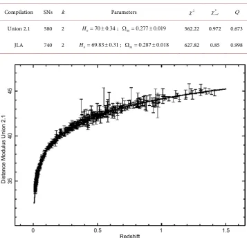
Compilation SNs k Parameters χ2 2

red

χ Q

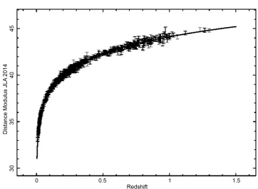
Union 2.1 580 2 H0=70±0.34; Ω =M 0.277±0.019 562.22 0.972 0.673 JLA 740 2 H0=69.83 0.31± ; Ω =M 0.287±0.018 627.82 0.85 0.998

Figure 1. Hubble diagram for the Union 2.1 compilation. The solid line represents the best fit for the exact distance modulus in flat cosmology as represented by Equation (7), parameters as in first line of Table 1.

The above equation takes a simple expression when the minimax rational approxi-mation is used, see [4][16] [17]; here we have used a polynomial of degree 3 for the numerator and degree 2 for the denominator. With the parameters of Table 1 for the Union 2.1 compilation over the range in z∈

[ ]

0, 4 , we obtain the following minimax

approximation

(

)

3,2,10 2 2 3

0.413991 6.080622 5.501967 0.029254 0.012154 0.148352 0.112017

z z z

m M

z z

+ + +

− =

+ + (21)

the maximum error being 0.002956.

3. Conclusion

[image:5.595.193.556.59.325.2]

Figure 2. Hubble diagram for the JLA compilation. The solid line represents the best fit for the exact distance modulus in flat cosmology as represented by Equation (7), parameters as in second line of Table 1.

A simple expression for the distance modulus relative to the Union 2.1 compilation is given through the minimax approximation applied to a Taylor expansion of the lumi-nosity distance of order 10.

References

[1] Pen, U.L. (1999) Analytical Fit to the Luminosity Distance for Flat Cosmologies with a Cosmological Constant. Astrophysical Journal Supplement Series, 120, 49.

http://dx.doi.org/10.1086/313167

[2] Adachi, M. and Kasai, M. (2012) An Analytical Approximation of the Luminosity Distance in Flat Cosmologies with a Cosmological Constant. Progress of Theoretical Physics, 127, 145. http://dx.doi.org/10.1143/PTP.127.145

[3] Mészáros, A. and Řpa, J. (2013) A Curious Relation between the Flat Cosmological Model and the Elliptic Integral of the First Kind. Astronomy & Astrophysics, 556, A13.

http://dx.doi.org/10.1051/0004-6361/201322088

[4] Olver, F.W.J., Lozier, D.W., Boisvert, R.F. and Clark, C.W. (2010) NIST Handbook of Ma-thematical Functions. Cambridge University Press, Cambridge.

[5] Abramowitz, M. and Stegun, I.A. (1965) Handbook of Mathematical Functions with For-mulas, Graphs, and Mathematical Tables. Dover, New York.

[7] Garnavich, P.M., Kirshner, R.P., Challis, P., Tonry, J., Gilliland, R.L., Smith, R.C., Cloc-chiatti, A., Diercks, A., Filippenko, A.V., Hamuy, M., Hogan, C.J., Leibundgut, B., Phillips, M.M., Reiss, D., Riess, A.G., Schmidt, B.P., Schommer, R.A., Spyromilio, J., Stubbs, C., Suntzeff, N.B. and Wells, L. (1998) Constraints on Cosmological Models from Hubble Space Telescope Observations of High-z Supernovae. Astrophysical Journal Letters, 493, L53. http://dx.doi.org/10.1086/311140

[8] Riess, A.G., Filippenko, A.V., Challis, P. and Clocchiatti, A. (1998) Observational Evidence from Supernovae for an Accelerating Universe and a Cosmological Constant. Astronomical Journal, 116, 1009. http://dx.doi.org/10.1086/300499

[9] Knop, R.A., Aldering, G., Amanullah, R., Astier, P., Blanc, G., Burns, M.S., Conley, A., Deustua, S.E., Doi, M., Ellis, R., Fabbro, S., Folatelli, G., Fruchter, A.S., Garavini, G., Gar-mond, S., Garton, K., Gibbons, R., Goldhaber, G., Goobar, A., Groom, D.E., Hardin, D., Hook, I., Howell, D.A., Kim, A.G., Lee, B.C., Lidman, C., Mendez, J., Nobili, S., Nugent, P.E., Pain, R., Panagia, N., Pennypacker, C.R., Perlmutter, S., Quimby, R., Raux, J., Reg-nault, N., Ruiz-Lapuente, P., Sainton, G., Schaefer, B., Schahmaneche, K., Smith, E., Spada-fora, A.L., Stanishev, V., Sullivan, M., Walton, N.A., Wang, L., Wood-Vasey, W.M. and Yasuda, N. (2003) New Constraints on ΩM, ΩLambda, and w from an Independent Set of 11 High-Redshift Supernovae Observed with the Hubble Space Telescope. Astrophysical Journal Letters, 598, 102. http://dx.doi.org/10.1086/378560

[10] Riess, A.G., Strolger, L.G., Casertano, S., Ferguson, H.C., Mobasher, B., Gold, B., Challis, P.J., Filippenko, A.V., Jha, S., Li, W., Tonry, J., Foley, R., Kirshner, R.P., Dickinson, M., MacDonald, E., Eisenstein, D., Livio, M., Younger, J., Xu, C., Dahlén, T. and Stern, D. (2007) New Hubble Space Telescope Discoveries of Type Ia Supernovae at z Greater than 1: Narrowing Constraints on the Early Behavior of Dark Energy. Astrophysical Journal Let-ters, 659, 98. http://dx.doi.org/10.1086/510378

[11] Suzuki, N., Rubin, D., Lidman, C., Aldering, G., Amanullah, R., Barbary, K. and Barrientos, L.F. (2012) The Hubble Space Telescope Cluster Supernova Survey. V. Improving the Dark- Energy Constraints above z Greater than 1 and Building an Early-Type-Hosted Supernova Sample. Astrophysical Journal Letters, 746, 85.

http://dx.doi.org/10.1088/0004-637X/746/1/85

[12] Betoule, M., Kessler, R., Guy, J. and Mosher, J. (2014) Improved Cosmological Constraints from a Joint Analysis of the SDSS-II and SNLS Supernova Samples. Astronomy & Astro-physics, 568, A22. http://dx.doi.org/10.1051/0004-6361/201423413

[13] Oliveira, F.J. (2016) Cosmic Time Transformations in Cosmological Relativity. Journal of High Energy Physics, Gravitation and Cosmology, 2, 253.

http://dx.doi.org/10.4236/jhepgc.2016.22022

[14] Press, W.H., Teukolsky, S.A., Vetterling, W.T. and Flannery, B.P. (1992) Numerical Recipes in Fortran. The Art of Scientific Computing. Cambridge University Press, Cambridge. [15] Zaninetti, L. (2016) Pade Approximant and Minimax Rational Approximation in Standard

Cosmology. Galaxies, 4, 4. http://www.mdpi.com/2075-4434/4/1/4

[16] Remez, E. (1934) Sur la détermination des polynômes d’approximation de degré donnée. Comm. Soc. Math. Kharkov, 10, 41.

Submit or recommend next manuscript to SCIRP and we will provide best service

for you:

Accepting pre-submission inquiries through Email, Facebook, LinkedIn, Twitter, etc. A wide selection of journals (inclusive of 9 subjects, more than 200 journals)

Providing 24-hour high-quality service User-friendly online submission system Fair and swift peer-review system

Efficient typesetting and proofreading procedure

Display of the result of downloads and visits, as well as the number of cited articles Maximum dissemination of your research work