Uncertainty and Heterogeneity in Returns to Education: Evidence from Finland

Munich Personal RePEc Archive

Uncertainty and Heterogeneity in

Returns to Education: Evidence from

Finland

Kässi, Otto

University of Helsinki, Hecer

31 December 2012

Online at

https://mpra.ub.uni-muenchen.de/48738/

Uncertainty and Heterogeneity in Returns to

Education: Evidence from Finland

∗

Otto Kässi

June 2013

Abstract

This paper studies the causal effect of education on income uncertainty using a broad measure of income which encompasses unemployment risk. To accomplish this, the variance of residuals from a Mincer-type income regression is decomposed into unobserved heterogeneity (known to the individuals when making their educational choices) and uncertainty (un-known to the individual). The estimation is done using Finnish registry data. The marginal effect of having secondary or lower tertiary level ed-ucation decreases income uncertainty. University level eded-ucation is found to have a small positive marginal effect on income uncertainty. The ef-fect of education on income uncertainty is roughly similar for men when compared to women, but income uncertainty is larger for men than for women regardless of education. Contrary to some results from the U.S., the role of unobserved heterogeneity is found to be very small.

JEL: C35, J31

Keywords: earnings uncertainty, unobserved heterogeneity, permanent variance, transitory variance

∗_{I am thankful to Bent Jesper Christensen, Gero Dolfus, Kristian Koerselman, Anssi}

Ko-honen, Tomi Kyyrä, Tuomas Pekkarinen, Roope Uusitalo, Tatu Westling and the participants of the HECER Labor Economics Workshop 2012, HECER Economics of Education Summer Meeting 2012 and Aarhus University Economics Brown Bag seminar for various useful com-ments. Financial support from Kone Foundation, Yrjö Jahnsson Foundation and OP Pohjola Foundation is gratefully acknowledged. A part of this work was completed when I was visiting Aarhus University. I am grateful for their hospitality.

1

Introduction

Return to education is perhaps the most widely studied causal relationship in contemporary economic literature. A central message from this literature is that measuring monetary return to education is complicated by endogenous selection. Endogenous selection arises simply from the fact that people who choose different levels of education levels are likely to differ from one another in some dimensions unobservable to the researcher. Neglecting this unobserved heterogeneity may potentially introduce a large bias.

Monetary uncertainty in return to education has received much smaller em-pirical attention. Since the return to education is not constant among indi-viduals and materializes possibly only several years after the choice of educa-tion has been made, educaeduca-tional investment has an inherent uncertainty to it. Analogously to estimating mean returns to education, endogenous selection also complicates the estimation of uncertainty in monetary returns to education.

The measure of earnings uncertainty used throughout this paper is the vari-ance of yearly income. For example, a direct comparison of income varivari-ances between university and high school educated people might give an incorrect pic-ture of the effect of education on income variance, because we cannot observe counterfactual income streams of the same people with different education lev-els. Consequently, the observed variance of income may not be a good measure of uncertainty, because it is comprised of two distinct components: unobserved heterogeneity and uncertainty. The intuition for this dichotomy follows from private information: wage uncertainty, or risk, is the part of the wage variance, which is not foreseeable by the decision-maker.

Unobserved heterogeneity (due to, for example, individual ability, motivation and general taste for education), on the other hand, is the portion of the wage variance which is known to – and acted on by – the individual, but not observed by the researcher. The unobserved heterogeneity is intimately related to private information on potential returns to education possessed by individuals. For example, if a person knows that her personal return from a given education level is particularly high, she will most likely choose that level of education. Disentangling unobserved heterogeneity (which stems from private information) from true uncertainty from the point of view of the agent making the schooling decision is instrumental when studying income uncertainty.

This paper studies two interrelated decompositions. First, I correct for self-selection by modeling the self-selection of education level. Second, I decompose the uncertainty of income into a permanent component, which reflects fixed charac-teristics of individuals and a transitory component, which reflects idiosyncratic shocks to income streams of individuals. The transitory component is allowed to vary by time and by education level.

I follow Chen (2008) who extends the framework of Roy (1951) into more than two sectors. Chen disentangles potential variance and unobserved hetero-geneity from one another, while taking into account the fact that the selection of agents into educational categories is endogenous. Chen estimates her model using data on U.S. males. She finds that the uncertainty-education profile is U-shaped; the most and least educated individuals face the highest income un-certainty. In addition, according to her model, unobserved heterogeneity is estimated to be up to 20 percent of the total earnings uncertainty.

The dependent variable in Chen’s paper is average hourly wage. Her ap-proach disregards perhaps the most important source of earnings uncertainty; namely, the risk of unemployment. Instead of hourly wages, this paper studies yearly total taxable income, which, in addition to income from employment, includes unemployment benefits and other taxable transfers. This measure ar-guably gives a more complete picture of the income uncertainty related to a level of education. This is particularly relevant because international evidence suggests that differences in unemployment risks between education groups may be substantial (Guiso et al., 2002) and have widened in recent decades (Ace-moglu & Autor, 2011). Using total taxable income as the measure of income also mitigates the problem of endogenous selection into employment, as people are observed even if they are not working. The model presented in this paper is estimated using Finnish data. An attractive featur e of the Finnish tax code for the current purposes is that virtually all of the income transfers, including unemployment benefits, are taxable and are therefore observed.

I also depart from Chen’s approach in another way. Namely, I estimate sep-arate models for men and women. In most similar studies attention is limited to men, because female workforce participation in most countries has been much lower until recent years. Nonetheless, the female workforce participation in Fin-land has been similar to male workforce participation already from the 1990s, which warrants doing a similar analysis also for females. Furthermore, since both female education and female workforce participation has also increased in-ternationally, I find that calculating comparable measures for males and females is also interesting in its own right from an international perspective. As a result, I am able to test whether there are differences in the amount of uncertainty in career paths between men and women.

an appropriate instrument, which affects schooling but does not appear in the income equation, is needed. I use local differences in supply of education proxied by the region of residence in youth as an instrument. Even though I am able to control for a wealth of family background and individual characteristics, endogeneity of the instrument can not be ruled out. It turns out, that even an analysis using a possibly endogenous instrument is informative.

The association between mean earnings and its variance has been studied, among others, by Palacios-Huerta (2003), Hartog & Vijverberg (2007), Diaz-Serranoet al.(2008) and Schweri et al. (2011). The aforementioned papers do not find any robust relationship between education group income means and variances. This may be related to the fact that none of these papers address the possible selection effects.

In addition, the current paper nests two other prominent research themes. First, I explicitly allow for heterogeneity in the return to education. In this sense, the approach of paper is related to models used to study heterogeneous returns to schooling (e.g. Aakviket al.2010 and Abadieet al.2002). Second, the approach chosen here is related to Cunha & Heckman (2008), Cunhaet al.(2005) and Cunha & Heckman (2007), all of which study how the private information of individuals is related to their choice of education, but do not discriminate between permanent and transitory components. The approach of Chen (2008) is also applied in Mazza & van Ophem (2010) and Mazzaet al. (2011).

As a preview of the results, I find that income uncertainty decreases up to the tertiary level of education. University educated individuals face slightly larger earnings uncertainty compared to people with a tertiary level education. For men, however, this effect is not distinguishable from zero. In addition, men face higher income uncertainty in comparison to women regardless of their education levels. Moreover, the estimates for the role of unobserved heterogeneity are found to be very small compared to estimates from the U.S.

2

Brief description of the education system in

Finland

The Finnish system of education consists of three stages. The first stage is compulsory education (9 years), which gives eligibility to apply for a secondary education. Secondary education (3 years) is provided by academically oriented upper secondary and vocational secondary schools. After completing secondary education, people apply to tertiary education (3-5 years), which is offered in universities (master’s level) and polytechnic colleges (lower tertiary level).

There are two stages of selection. First one takes place after comprehensive school when students are about 16 years old. Students have an opportunity to apply to an academically oriented upper secondary school or to a more practi-cally oriented vocational school. The second stage of selection takes place when people apply for tertiary education. In addition to upper secondary school graduates, also vocational school graduates are allowed to apply for tertiary education.

Tertiary education is offered in universities and polytechnic colleges. The focus of universities is research whereas polytechnic colleges are more practi-cally oriented. Graduates from polytechnics are able to apply to universities to continue their studies. There are no tuition fees at any level. In addition, a student benefit of roughly EUR 400 monthly is offered to students over 18 not living with their parents.

I use a categorical education measure, Si, with four distinct categories to

capture the salient features of the Finnish education system. Each individuali, is placed into one of the schooling categories, which are

• Si= 1; compulsory education,

• Si= 2; secondary education (both vocational and upper),

• Si= 3; lower tertiary education,

• Si= 4; university level education.

As the data does not allow me to identify dropouts, I classify people according to their highest completed level of education.

3

Empirical model

3.1

Model for potential incomes

The stylized model consists of two periods. In the first period, individuals choose their levels of education according to their tastes. In the second period, they face a yearly income stream which depends on the level of education they have chosen and gets an income stream which depends on personal characteris-tics (both observed and unobserved) and education and time specific transitory and permanent shocks. I observe a panel ofN workers overT years. In the first observation year each worker has already chosen and completed their preferred level of education. The potential log-income of personiwith schoolingsin year

tis given by

ysit =yitI(Si= 1) +yitI(Si= 2) +yitI(Si = 3) +yitI(Si= 4), (1)

whereI(·)is an indicator function having a value of 1if Si=s (s= 1,2,3,4)

and0 otherwise. The potential wage formulated in (1) gives rise to an income regression equation of the form:

ysit=αs+xitβ+σsesi+ψstεit, ∀Si=s. (2)

In (2)αsis the mean earnings for a schooling level andxitis a vector of

observ-ables. The error term consists of two parts. The time invariant fixed effects are incorporated inσsesi. ψstεitdenotes transitory shocks, which are assumed to be

uncorrelated with both the observable characteristics and the fixed effect. The potential wage variance within a schooling level in yeart is thereforeσ2

s+ψst2.

Variation inσ2

s is the variance of individual specific fixed effects that are

con-stant in time but may vary across schooling levels. ψstεit, on the other hand,

may vary with both time and schooling level. esi and εit are assumed to be

N(0,1)distributed random variables.

It is assumed, that each individual chooses their level of education according to their preferences. This is formalized by a standard latent index model

S∗

i =ziθ+vi, (3)

whereS∗

i represents the optimal level of schooling chosen by individual i. The

latent schooling factorvi is aN(0,1) random variable. It summarizes the

pri-vate information such as taste for education, unobservable ability and income expectations (including possible risk aversion), which are known to the individ-ual but unobservable to the researcher.1

zi contains the elements in vector xi

and an instrument, which is assumed only to affect level of education but not income.

1

In particular,viis assumed to capture both pecuniary and non-pecuniary utility

The predicted schooling levelSi depends on Si∗ by

Si= 1 if −∞< ziθ+vi≤κ1,

.. .

Si= 4 if κ4≥ziθ+vi>∞.

(4)

The cutoff value,as=κs−ziθ, is the minimal level of the unobserved schooling

factor for which individuals chooses.

The model has three unobservable elements,esi, εitandvi.They are assumed

to be jointly normal with the structure

  esi εit vi 

 ∼ N

    0 0 0  ,  

1 0 ρs

0 1 0

ρs 0 1  



, (5)

whereρs∈[−1,1].Intuitively (5) implies that the unobservables in the

school-ing equation may be correlated with permanent earnschool-ings differences, but they are assumed to be uncorrelated with the transitory shocks. Therefore, the pos-sible selection bias only contaminates the estimation of the permanent com-ponent. The transitory component captures macroeconomic shocks and insti-tutional changes which affect all individuals symmetrically and are therefore uncorrelated withvi.The structure of the unobservables is assumed to be

com-mon knowledge2

.

Correlation between the fixed effect and the unobserved schooling factorρs

has a central role in the model: it captures the selection effect. If ρs > 0,

the unobservables in schooling and earnings equations are positively correlated, the selection effect is positive and workers with high income potential get more education. If ρs < 0, people with high income potential tend to enter labor

markets at a younger age. Consequently, ρs also governs the magnitude and

the direction of the bias in the OLS estimates: if ρs >0, OLS overstates the

true return to education and if ρs < 0, OLS understates the true return to

education.3

From the point of view of an individual making her schooling decision, the expected log-income is given by

E[ysit|si=s, xit, vi] =αs+xitβ+σsρsvi, (6)

2

The assumption of common knowledge of shock parameters is needed for the subsequent analysis. Even though this assumption might seem unrealistic, results from survey data (e.g.

Schweriet al._{, 2011 and Webbink & Hartog, 2004) and structural models (e.g. Charles &}

Luoh, 2003) support the assumption that students have at least some knowledge of their potential post-schooling income.

3

Cameron & Heckman (1998) discuss, which types of economic models would rationalize the ordered structure given by Equations (3), (4) and (5). Most importantly, they conclude

where the termσsρsvirepresents the channel through which individual schooling

factors affect the potential wage.

Since agents are assumed to know their own draw of vi, a proper measure

of income uncertainty should account for vi. The unforeseeable component of

log-income, or income uncertainty from the point of view of an individual, is measured by the deviation of realized income from its mean conditional on unobservablevi and observablesxit andSi

τ2

st = V ar[σsesi+ψstεei|xit, Si=s, vi]

= σs2 1−ρ 2 s

+ψ2st. (7)

Equation (7) can be rearranged to σ2 s +ψ

2 st = σ

2 sρ

2 s+τ

2

st. It shows that the

residual variance of equation (2) consists of two parts: unobserved heterogene-ity(σ2

sρ2s)and uncertainty(τst2). Income uncertainty is governed by the

perma-nent and transitory compoperma-nents (σs and ψst) and the correlation between the

unobserved schooling factor and permanent componentρs.

3.2

Identification of variance components

Equations (6) and (7) are not directly applicable for regression analysis because

vi is unobservable. To account for the effect of unobserved vi, a multi-choice

version of the Heckman selection correction model (Heckman, 1979) is used. As a first stage, a latent index model (3) is estimated using ordered probit. The model is used to calculate generalized residuals of the schooling model4

,

λsi=

φ(κs−ziθ)−φ(κs+1−ziθ)

Φ (κs+1−ziθ)−Φ (κs−ziθ)

,

whereφ(·)is the probability density function of a standard normal distribution and Φ (·) is the cumulative distribution function of a standard normal distri-bution. Adding λsi as a regressor to (6) accounts for the correlation between

unobserved schooling factor and education level. The expected value of observed wages from the point of view of the researcher can now be written as

E[ysit|si=s, xit, vi] =αs+xitβ+σsρsλi. (8)

Calculating the difference between realized and expected wages gives

ysit−E[ysit|si=s, xit, vi] =σs−σsρs+ψst. (9)

Variance of (9) equals the measure of uncertainty, τ2

st. Additionally, (9)

im-plies that whenever ρs 6= 0, selection leads to a truncation of the observed

in-come variance which, in turn, leads to an understatement of inin-come uncertainty

4

compared to the case we would observe if education was randomly assigned to individuals. The degree of understatement is given by5

:

δsi=λ2si−

(κs−ziθ)φ(κs−ziθ)−(κs+1−ziθ)φ(κs+1−ziθ)

Φ (κs+1−ziθ)−Φ (κs−ziθ)

.

The variance of transitory component can be identified from the residuals of the within-individual model,

(yit−y¯i) = (xit−x¯i)β− ξsit−ξ¯si

, (10)

where bars denote time averages of the corresponding variables (note that time-invariant individual regressors, includingλsi, are subsumed in the fixed effects)

and ξsit = ψstεsit. The procedure for estimating ψˆst2 is discussed in detail in

Appendix A.

The regression coefficients αˆs,βˆ and ρsˆσs = ˆγs can be identified using a

between-individuals model

¯

yi=αs+ ¯xiβ+γsλ¯si+ωi. (11)

The error term in (11) is, by equation (9),

ωi = σsesi+ ¯ξsi−γsλsi,

and its variance is

V ar[ωi|Si=s] =σs2−γ 2

sδsi+ψst2

Solving this for σ2

s gives the estimator for time invariant individual specific

variance of wages for each schooling level,

ˆ

σs2=V ard[ωi|Si=s] + ˆγs2δ¯ˆs−ψˆ2st, (12)

where, again, bars denote averages over individuals. The second termγˆ2 s

¯ ˆδsin

equation (12) is needed to correct for the truncation of variances due to self selection. Each term in equation (7) is now identified:

ˆ

τ2 st= ˆσ

2 s−γˆ

2 s+ ˆψ

2

st (13)

4

Data

The data used in this paper is a random sample of 46321 individuals from a Finnish Census. I limit my attention to working males and females aged between 28 and 43. I assume that by the age of 28, people have finished their

5_λ

education. An educational category of an individual is defined as the education they have at the youngest age they are observed in the panel. It is possible that individuals educate themselves further after the age of 28, but as my main interest is, how well individuals are able to predict their income in their youth, I interpret individuals’ decision to re-educate themselves at later ages as a realized uncertainty, which should not be controlled for.6

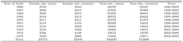
The panel spans 1994-2009, adding up to a total of 244637 individual-year observations for men and 213840 for women. The composition of the sample is summarized in Table 1. The panel is constructed in a way that even the youngest cohort is observed for six years. I have limited my attention to in-dividuals who were born after 1966 to make sure that an educational reform which took place in Finland in the early 1970’s does not differently affect the cohorts under study.7

The educational categories are defined according to the standard classifica-tion of educaclassifica-tion. I do not discriminate between fields of educaclassifica-tion but only levels as the goal of this paper is to study the returns of an attained degree rather than returns to years of education. The specification used allows the marginal return to schooling to vary according to the level of schooling completed. Us-ing the highest degree attained also mitigates the effect of measurement errors, since years of education are usually imputed using average years of education needed to complete a degree, which introduces measurement error.

As already mentioned, the risk of unemployment constitutes a considerable part of the total income uncertainty. The choice of the outcome variable reflects this; the dependent variable in income regressions is the log of total yearly tax-able income which, in addition to wages and entrepreneurial income, includes taxable income transfers but excluding income from capital gains. As a result, the observed income streams allow for potential spells of unemployment.8

How-ever, if a person drops out of the workforce entirely, she only contributes to the estimation for the years when she is either unemployed or working. The variance of yearly total income is, by definition, comprised of three components, hourly wages, hours worked and the means-tested income transfers. Consequently, un-less the covariances of the three components are very large and negative, the total variances will be higher than the variance of hourly wages (see, e.g. Abowd

6

In practice this is rather rare. Only roughly five percent of individuals in the lowest education category get a higher degree during the time in the panel. For higher education categories, the proportion of people who re-educate themselves are in the order of 1 percentage.

7

The goal of this reform was to standardize the quality of comprehensive education within the country. Consequently, people born before 1966 had a different school system from those born after 1966. In particular, before the reform, the quality of comprehensive education varied a great deal between regions. In addition, the reform resulted in removal of one educational

tracking stage. For details about the reform, see e.g., Pekkarinenet al._(2009).

8

& Card 1989).9

The income concept may introduce a problem of its own, since not working may be either voluntary or involuntary. To separate the involuntarily unem-ployed from voluntary workforce non-participants I include only the observations where the main type of activity of an individual is either working or unemployed in the estimation10

. For example, if a women is on a maternity leave for one year, but is either working or unemployed for nine years, she contributes to the estimation for the years when she is not on a maternity leave.

The approach chosen leaves some (likely mis-classified) observations with zero income. I omit these observations. This does not affect the main results, because the proportion of zero-observations is very small (less than 2% of ob-servations)11

. To ensure comparability between years, the measure of income is deflated to EUR 2009 using the Consumer Price Index.

I do not have a reliable information on whether workers are part-time or full-time. Therefore, to some extend, the uncertainty measures also reflect voluntary part-time work. Nonetheless, the proportion of part-time workers is rather small in comparison to most developed countries. The proportion of part-time workers is 9.2% for men and 16.9% for women. Further, working part-time is virtually nonexistent in professional and management positions (where most peopleare likely in education categories 3 or 4) (Eszter, 2011).

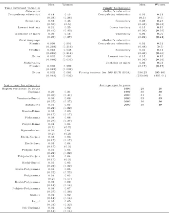
The vector of controls in Equation (2) includes paternal and maternal ed-ucation classified using the same four-level classification which is used for in-dividuals’ own education, a measure for family income calculated as the sum the income of mother and income of father and nine dummies for family socioe-conomic status. Family background characteristics are measured at age 14 if possible. In addition, controls for first language, nationality and the region of residence in adulthood are included.

Estimation of Equation (11) necessitates an instrument excluded from the income equation (2). The region of residence in youth is used as an instru-ment.12 13

The assumption is that the region of residence is correlated with individuals’ access to higher education but not their income after controlling for

9

Lowet al._{(2010) discuss a model which separates individual productivity and firm-worker}

match specific unemployment risks from one another in a structural framework. The depen-dent variable in this paper, total taxable income, should be interpreted as a combination of productivity and match specific risks, but measuring the respective contributions of these two parts is beyond the scope of this paper.

10

In general, for an individual to be classified as unemployed (and be eligible for unemploy-ment benefits), she must agree to accept a job if offered one.

11

None of the results qualitatively change whether I exclude them or impute a small positive income value for these observations.

12

Childhood information is collected from censuses. Censuses were administered in 1970, 1975, 1980, 1985 and yearly from 1988 onwards.

13

A similar instrument is used, among others, by Suhonenet al._{(2010) for Finland, Card}

other observable characteristics. Consequently I need to exclude individuals who have no information on their place of residence at youth. The estimation results provided in Section 4.1 support the notion that the instrument is relevant.

As discussed by Card (1993), the place of residence in youth may affect income because of differences in local supply of education, but also because family background is correlated with place of residence. For this reason family background variables are controlled for. In addition, Card points out that dif-ferences in comprehensive schooling resources may affect subsequent income. In the case of Finland, comprehensive education is arranged in public schools with very small differences in resources and quality (Kirjavainen, 2009). In addition, international evidence suggests that the impact of school quality on learning (Kramarz et al., 2009) and income (Betts, 1995) is rather small even in the context of less standardized comprehensive schooling. Finally, to control for differences in local labor market conditions in the presence of imperfect labor mobility, I control for job location in adulthood in the income equation. Despite controlling for family background and job location characteristics, it might still be the case that the instrument is correlated with the outcome. If this is the case, the estimates forρsoverestimate the true parameter value. I discuss this

possibility in Section 6.

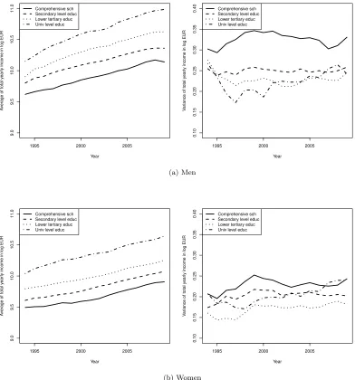
Figure 1 plots the estimated averages and standard deviations of log incomes for each panel year calculated from the sample described in Table 2. It is apparent that the mean income rises with education. Differences in the standard deviations of incomes are quantitatively much smaller, but some aspects can already be noted. First, people with only a compulsory education have the largest standard deviations of incomes. The standard deviation of male income in the lowest education category is especially large. The relative contribution of heterogeneity, permanent differences and transitory differences remains unclear. Using the method outlined in the previous section, it is possible to disentangle them from one another

Control variables, which capture the observed heterogeneity, are summarized in Table 2. Not surprisingly, the distribution of family background variables is virtually identical between sexes. There are larger differences in the distribution of education levels. The proportion of men with a basic or secondary education is larger than women. Conversely, there are more women with at least a tertiary level education.14

14

1995 2000 2005 9.0 9.5 10.0 10.5 11.0 Year A ver

age of total y

ear

ly income in log EUR

Comprehensive sch Secondary level educ Lower tertiary educ Univ level educ

1995 2000 2005

0.10 0.15 0.20 0.25 0.30 0.35 0.40 Year V ar

iance of total y

ear

ly income in log EUR

Comprehensive sch Secondary level educ Lower tertiary educ Univ level educ

(a) Men

1995 2000 2005

9.0 9.5 10.0 10.5 11.0 Year A ver

age of total y

ear

ly income in log EUR

Comprehensive sch Secondary level educ Lower tertiary educ Univ level educ

1995 2000 2005

0.10 0.15 0.20 0.25 0.30 0.35 0.40 Year V ar

iance of total y

ear

ly income in log EUR

Comprehensive sch Secondary level educ Lower tertiary educ Univ level educ

(b) Women

Table 1: Sample sizes used in estimation.

Year of birth Sample size (men) Sample size (women) Year-obs. (men) Year-obs. (women) Years

1966 2742 2543 38576 33335 1994-2009

1967 2696 2510 35330 30382 1995-2009

1968 2530 2501 31253 28601 1996-2009

1969 2318 2213 26752 23623 1997-2009

1970 2417 2211 25729 21475 1998-2009

1971 2118 2155 20589 19216 1999-2009

1972 2134 2056 18905 16643 2000-2009

1973 2100 1928 16462 13915 2001-2009

1974 2226 2146 15612 13739 2002-2009

1975 2492 2285 15429 12911 2003-2009

Total 23773 22548 244637 213840

5

First and second stage estimates

5.1

First stage: schooling choice

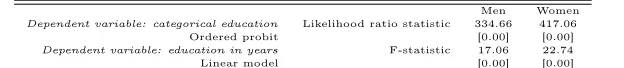
Equation (3) is estimated by an ordered probit. The estimated model includes family background measures and the instrument for education. Table 3 shows the test statistics for the relevance of the instruments. The relevance of instru-ment using linear education as the dependent variable is also reported because there are no rule-of-thumb test statistic values for the relevance of instruments maximum likelihood models.. Educational categories are converted to years of education using average times-to-degree measured in full years.15

This intro-duces noise to the dependent variable. Consequently the F-statistics reported in Table 3 might represent a lower bound for the effect of the instruments on education. Nonetheless, even the F-statistics of the linear model suggest that the instruments are highly relevant.

5.2

Second stage: average returns to schooling

This section presents estimates for the average returns to education. The re-ported estimates are based on the between model (11), where average yearly income of an individual is regressed on individual characteristics, schooling vari-able, mean age, mean age squared and the generated regressorλsi.

To account for the fact thatλsiis a generated regressor, the standard errors

are calculated using a block bootstrap procedure, where 200 samples of size

N are drawn with replacement from the original population. For each boot-strap drawk, the estimatesαˆk

s,βˆ k

andγˆk

s are calculated. Expected values and

standard errors of the parameters are calculated from the distribution of these bootstrap draws.

The parameter estimates and their standard errors are presented in the sec-ond column of Table 4. The effect of education on income is nonlinear with

15

Table 2: Descriptive statistics of the explanatory variables.

Men Women Men Women

Time invariant variables Family background

Education Father’s education

Compulsory education 0.18 0.15 Compulsory education 0.53 0.53

(0.38) (0.36) (0.5) (0.5)

Secondary 0.52 0.45 Secondary 0.25 0.25

(0.50) (0.5) (0.43) (0.43)

Lowest tertiary 0.21 0.25 Lower tertiary 0.15 0.15

(0.41) (0.43) (0.36) (0.36)

Bachelor or more 0.09 0.16 University 0.06 0.06

(0.29) (0.37) (0.24) (0.24)

First language Mother’s education

Finnish 0.950 0.951 Compulsory education 0.52 0.52

(0.218) (0.216) (0.48) (0.5)

Swedish 0.048 0.048 Secondary 0.31 0.31

(0.215) (0.214) (0.46) (0.46)

Other 0.002 0.001 Lowest tertiary 0.15 0.15

(0.040) (0.032) (0.36) (0.36)

Nationality Bachelor or more 0.03 0.03

Finnish 0.998 0.999 (0.17) (0.17)

(0.042) (0.032)

Other 0.002 0.001 Family income (in 100 EUR 2009) 394.23 393.401 (0.042) (0.032) (253.06) (253.01)

Instrument for education Average ages in years

Region residence in youth 1994 28 28

Uusimaa 0.20 0.21 1997 30 30

(0.40) (0.41) 2000 31 31

Varsinais-Suomi 0.08 0.08 2003 33 33

(0.27) (0.27) 2006 36 36

Satakunta 0.05 0.05 2009 39 39

(0.22) (0.22) Kanta-Häme 0.03 0.03

(0.17) (0.17) Pirkanmaa 0.08 0.08

(0.27) (0.27) Päijät-Häme 0.04 0.04

(0.2) (0.2) Kymenlaakso 0.04 0.04 (0.2) (0.2) Etelä-Karjala 0.03 0.03 (0.17) (0.17) Etelä-Savo 0.03 0.04

(0.17) (0.2) Pohjois-Savo 0.05 0.05 (0.22) (0.22) Pohjois-Karjala 0.03 0.04

(0.17) (0.2) Keski-Suomi 0.05 0.05 (0.22) (0.22) Etelä-Pohjanmaa 0.05 0.05

(0.22) (0.22) Pohjanmaa 0.04 0.03

(0.2) (0.17) Keski-Pohjanmaa 0.02 0.02

(0.14) (0.14) Pohjois-Pohjanmaa 0.08 0.07

(0.27) (0.26) Kainuu 0.02 0.02

(0.14) (0.14) Lappi 0.05 0.05

(0.22) (0.22) Itä-Uusimaa 0.02 0.02

(0.14) (0.14)

Notes: Standard deviations in parentheses. Calculations are based on a random sample of individuals who are born between 1966–1975 and are between 28 and 43 years old.Nis the sample size of time-invariant variables.

Table 3: Test statistics for relevance of instrument.

Men Women Dependent variable: categorical education Likelihood ratio statistic 334.66 417.06

Ordered probit [0.00] [0.00] Dependent variable: education in years F-statistic 17.06 22.74 Linear model [0.00] [0.00] Notes: P-values in brackets. Instrument for education is the region of residence in youth. Both models include

controls for parents’ education, family income, nationality, first language and year of birth.

respect to level of education. Most educated individuals accrue the highest marginal returns.

To facilitate comparability to previous literature on monetary returns to education, also IV estimates for the average return to education are reported in the third column of Table 4. They are reported for reference, but are not used when estimating uncertainty parameters. The IV estimates are somewhat larger than the corresponding estimates based on the selection model.

Without selectivity correction, the positive correlation between schooling of individuals and the residual in the income equation would result in an upward bias in the estimated returns to income. This bias arises if some of the un-observable characteristics (a high draw of esi) are positively correlated with

the schooling choice of an individual. This happens, for example, if the people with high income potential are also those who self-select into higher education (Griliches, 1977).

In the context of the current model, the correlation between income and schooling presents itself in positive values of the correction termγs. There is

limited evidence of this: for men the estimate of the correction terms for lowest education categoriesγ1 andγ2and for the correction term for the highest

edu-cation categoryγ4for women are statistically significantly positive conventional

significance levels. The correction terms for other levels of schooling are not statistically distinguishable from zero at conventional levels. Even the correc-tion terms that differ statistically significantly from zero are qualitatively rather small. 16

The error structure given in Equation (5) implies that γs = ρsσs in

con-junction with the finding my estimate for ρˆ is very small suggests that the unobservable heterogeneity for each education level is very small. This implies that, either, individuals have very little private information on their compara-tive advantage not captured by the observable characteristics, or, alternacompara-tively, individuals do not act on their private information on potential incomes.

A possible concern for the validity of the results of this paper is that they hinge on the assumption of joint normality of error terms and the linear

depen-16

The fact that OLS and two-stage estimates are very close to one another, is a classic sign

of a weak instruments (e.g. Boundet al._{1995). Notice, however that the first stage results}

dence between mean incomes and the selection term. To shed some light on the concern, I have performed the test described in Vella (1998, pp. 137-138) and estimated Equation (11) where in addition to the Inverse Mills’ Ratio, second and third degree polynomials of the Inverse Mills’ Ratios are used as regressors. This allows me to test for possible deviations from joint normality of unobserv-ables in schooling and income equations. The tests for the joint significance of the higher order polynomial always fail to reject the null hypothesis of linearity. This speaks in favor of the assumption of the joint normality.

Confidence on the distributional assumptions is further strengthened by the fact that the estimates of|ρˆ| < 1 and ˆδsi ∈ [0,1] for all individuals, which is

consistent with normality (notice that no restrictions on ρˆ and ˆδ are placed). Nonetheless, even though the assumption of normality is not immediately re-jected, some caution should be exercised when interpreting the results, since they are obviously conditional on the distributional assumptions.

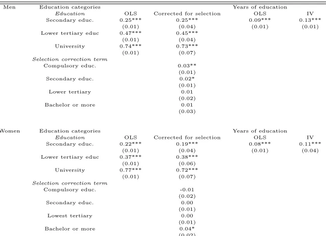
Table 4: Second stage estimates.

Men Education categories Years of education

Education OLS Corrected for selection OLS IV

Secondary educ. 0.25*** 0.25*** 0.09*** 0.13*** (0.01) (0.04) (0.01) (0.01) Lower tertiary educ 0.47*** 0.45***

(0.01) (0.04) University 0.74*** 0.73***

(0.01) (0.07) Selection correction term

Compulsory educ. 0.03** (0.01) Secondary educ. 0.02* (0.01) Lower tertiary 0.01

(0.02) Bachelor or more 0.01

(0.03)

Women Education categories Years of education

Education OLS Corrected for selection OLS IV

Secondary educ. 0.22*** 0.19*** 0.08*** 0.11*** (0.01) (0.04) (0.01) (0.04) Lower tertiary educ 0.37*** 0.38***

(0.01) (0.06) University 0.77*** 0.72***

(0.01) (0.07) Selection correction term

Compulsory educ. -0.01 (0.02) Secondary educ. 0.00

(0.01) Lowest tertiary 0.00

(0.01) Bachelor or more 0.04* (0.02)

Notes: Estimates are based on a between-individuals model. Standard errors in parenthesis. For the OLS and IV models, standard errors are based on the heteroskedasticity and autocorrelation consistent OLS covariance matrix. For the selection corrected model standard errors are based on 200 bootstrap replications. In addition to variables reported, both models include controls for parents’ education, family income, nationality, first language and year of birth, age and age squared. In columns 1 and 2, the education is measured as a categorical education variable.

6

Uncertainty estimates

6.1

Main estimates

The estimates for the permanent and transitory components of income uncer-tainty at each education level are reported in this section. Standard errors of each variance component are again calculated from 200 bootstrap resamples. The uncertainty estimates are reported in Table 5. Since the error structure assumed implies that unobserved heterogeneity is not correlated with the tran-sitory shocks, the total wage uncertainty is a sum of two components: trantran-sitory shocks and permanent earnings variance purged from the effects of private in-formation.

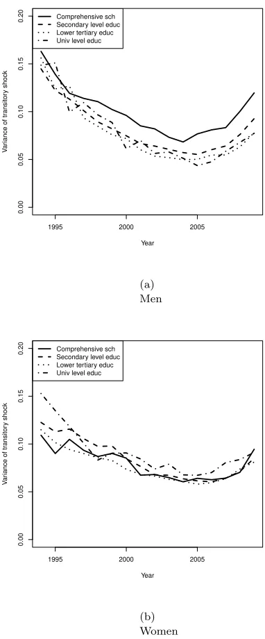
I first discuss the transitory variance estimates. Since transitory shocks are time-varying, I start by reporting the time-means of the transitory component (denoted byψ¯2

s). Among men, individuals in the lowest education group face

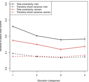
categories. Transitory and total income inequality levels are plotted in Figure 3.

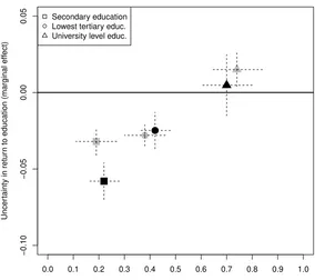
To get a better grasp of the effects of education on average return and un-certainty, Figure 4 plots the marginal effects of completed education on average income and income uncertainty. Completing a secondary education decreases income uncertainty of men more than that of women. A tertiary level education has a small negative effect on male and female earnings uncertainty. Completing an university level education increases uncertainty somewhat; this effect is, how-ever, statistically significant for men but not for women. The returns-to-degree estimates are similar among men and women on all levels of education.

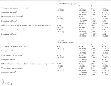
Table 5: Estimates of income variance components.

Men

Education category

1 2 3 4

Variance of transitory shock1 _{0.09 0.07 0.07 0.07}

(0.002) (0.001) (0.001) (0.002)

Marginal effects2 _{-0.02*** -0.001 0.001}

(0.002) (0.002) (0.003)

Permanent component3 0.17 0.13 0.11 0.11

(0.01) (0.01) (0.01) (0.01)

Marginal effects4 _{-0.04*** -0.02*** 0.00}

(0.006) (0.006) (0.01) Effect of private information on permanent component5 0.00 0.00 0.00 0.00

(0.06) (0.04) (0.04) (0.06) Total wage uncertainty6 0.26 0.20 0.18 0.18

(0.005) (0.003) (0.005) (0.009)

Marginal effects7 _{-0.06*** -0.02*** 0.01}

(0.006) (0.006) (0.01)

Women

Education category

1 2 3 4

Variance of transitory shock1 _{0.07 0.08 0.07 0.08}

(0.002) (0.001) (0.001) (0.002)

Marginal effect2 _{-0.002 -0.002* 0.005**}

(0.002) (0.001) (0.002)

Permanent component3 0.10 0.07 0.05 0.05

(0.004) (0.002) (0.002) (0.005)

Marginal effect4 _{-0.03*** -0.03*** 0.01}

(0.005) (0.003) (0.01) Effect of private information on permanent component5 _{0.00 0.00 0.00 0.00}

(0.04) (0.02) (0.02) (0.04) Total wage uncertainty6 0.17 0.15 0.12 0.13

(0.003) (0.002) (0.002) (0.005)

Marginal effect7 _{-0.03*** -0.03*** 0.01}

(0.004) (0.003) (0.05)

1_ψ¯2 s 2_ψ¯2

s−ψ¯2s−1

3_σ2 s 4_σ2

s-σ2s−1

5_γ2 s

6ψ¯2_s−γs2+σ2s=τ2s

7_τ2 s−τs2−1

Notes: Variance component decompositions are based on Equation (13) with region of residence in youth as an instrument. Standard errors from 200 bootstrap resamples in parenthesis. Education categories are: 1. compulsory

1995 2000 2005

0.00

0.05

0.10

0.15

0.20

Year

V

ar

iance of tr

ansitor

y shock

Comprehensive sch Secondary level educ Lower tertiary educ Univ level educ

(a) Men

1995 2000 2005

0.00

0.05

0.10

0.15

0.20

Year

V

ar

iance of tr

ansitor

y shock

Comprehensive sch Secondary level educ Lower tertiary educ Univ level educ

(b) Women

decreases

●

●

● ●

1 2 3 4

0.0

0.1

0.2

0.3

0.4

Education (categories)

V

ar

iance of y

ear

ly total income

●

●

● ●

●

●

●

●

● ●

●

● ●

●

●

●

Total uncertainty; men Transitory shock variance; men Total uncertainty; women Transitory shock variance; women

●

0.0 0.1 0.2 0.3 0.4 0.5 0.6 0.7 0.8 0.9 1.0

−0.10

−0.05

0.00

0.05

Mean return to education (marginal effect)

Uncer

tainty in retur

n to education (marginal eff

ect)

●

●

Secondary education Lowest tertiary educ. University level educ.

Figure 4: Marginal effects of completing a degree on mean income (horizontal axis) and uncertainty (vertical axis) for men (black symbols) and women (gray symbols). The dashed lines represent the bootstrapped 95% confidence intervals of return and uncertainty estimates on the corresponding axes.

6.2

Comparison to U.S. studies

that this is due to smaller risk of unemployment of more educated individuals. Perhaps a more surprising finding is the very small unobserved heterogene-ity. This is in stark contrast to the estimates based on data from the U.S.17

For example, Cunha & Heckman (2007) conclude that up to 50% of the ex post vari-ance in income of college graduates is attributable to unobserved heterogeneity, i.e. is foreseeable by individuals making their choice on whether or not to attend college. A potential explanation for the results is the choice of measure of in-come. The studies based on U.S. data use either a long period average earnings (Cunha & Heckman, 2007, 2008; Cunhaet al., 2005), or average hourly wage (Chen, 2008), which both arguably contain less variation than the yearly total income. Therefore, the correlation between residuals in schooling and income equations, which is used to identify unobserved heterogeneity, is mechanically smaller in absolute value.

A second partial explanation is that I target people in their youth. As the nine-year comprehensive school is mandatory, it may indeed be the case that young people making their choice on whether or not to attend higher education have limited information on their future incomes at the age of fifteen. In addi-tion, early-career earnings are usually more volatile, or more uncertain. Since the Finnish comprehensive education is extremely standardized and allows for little differentiation in school curricula between skill groups, it may convey less private information to students about their future incomes and, therefore lead to a smaller unobserved heterogeneity, than a less standardized system would.

However, even though the unobserved heterogeneity is found to be smaller than in the U.S., this does not necessarily imply that people would have less information on their potential future income streams. Rather, it seems plau-sible, that, given the high amount of redistribution and collective bargaining in Finnish labor market, people would have a rather good perception on their potential future income, but this perception is not correlated with individual characteristics which are unobservable to the econometrician.

6.3

Sensitivity of results to the instrument

Even though I control for a variety of background characteristics in both first and second stages, the validity of the instrument is somewhat questionable. It is possible that the instrument has a direct effect on income even after controlling for the elements ofx. To see the underlying intuition, note that the possibly

17

Mazzaet al._{(2011) attempts to replicate the results in Chen (2008) using the same data}

endogeneous instrument may affect the outcome through two distinct channels, through its independent effect on the probability of completing an education, and through direct effect of the instrument on income. More formally, the term

γs in equation (11) can be written as

γsλsi(ziθ, Si=s) =cov(vi, ωi |z,) +cov(ziγ, ωi|Si =s, xi). (14)

The first term in the expression is the correlation between the unobserved school-ing coefficient and the education. The second term is the covariance between income and the instrument when schooling and other observables except the instrument are kept constant. Equation (14) also provides a test for the ex-ogeneity of the instrument; in a sub-sample, where schooling is constant, the instruments should have no predictive power on income after controlling forx.

The tests for the joint significance of instruments are implemented separately for each schooling category and both sexes and reported in Table 6.

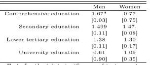
The instrument is found to have a direct effect to earnings in comprehensive schooling category for men and in the secondary education category for women. Consequently, for other education levels, the exogenous instrument assumption seems to hold. It should also be noted, that the endogeneity of the instrument biases the estimate ofρsupwardsin absolute value. Therefore, it seems plausible

that my estimates forρˆsrepresent an upper limit of the true parameter value.18

To further study, to what extend the possible endogeneity of instrument drives the results, I have estimated the model without an exclusion restriction. The estimation results are presented in tables 7 and 8. The results are very similar to those reported in Tables 4 and 5. Since the two alternative specifi-cations give very similar, and quantitatively small, estimates for the unobserved heterogeneity and, if anything, the main estimates are biased upwards in abso-lute value, it seems clear that unobserved heterogeneity is, indeed, very small.

Table 6: Test for the exogeneity of the instrument.

Men Women Comprehensive education 1.67* 0.77

[0.03] [0.75] Secondary education 1.499 1.47. [0.11] [0.08] Lower tertiary education 1.38 1.30

[0.11] [0.17] University education 0.61 1.09

[0.90] [0.35] Tests for the joint significance of instruments in samples with the same education. P-values in brackets.

18

Table 7: Second stage estimates (estimated without an exclusion restriction).

Men Education categories

Return to education level Corrected for selection Selection correction term Upper secondary educ. 0.25*** Comprehensive educ 0.00

(0.54) (0.01)

Lower tertiary educ 0.47*** Upper secondary educ. 0.00

(0.05) (0.01)

University 0.73*** Lower tertiary educ 0.00

(0.07) (0.02)

University 0.03* (0.02)

Women Education categories

Return to education level Corrected for selection Comprehensive educ 0.00 Upper secondary educ. 0.20*** (0.02)

(0.05) Upper secondary educ. 0.00 Lower tertiary educ 0.39*** (0.01)

(0.05) Lower tertiary educ 0.00

University 0.74*** (0.01)

(0.06) University 0.02 (0.02)

Notes: Estimates are based on a model without an instrument. Standard errors in parenthesis. Standard errors are based on 200 bootstrap replications. In addition to variables reported, both models include controls for location of residence, parents’ education and family income, nationality, first language and year of birth, age and age squared.

Table 8: Estimates of income variance components (estimated without an ex-clusion restriction).

Men

Education category

1 2 3 4

Variance of transitory shock1 0.09 0.07 0.07 0.07 (0.002) (0.001) (0.001) (0.002)

Permanent component2 _{0.17 0.12 0.10 0.10}

(0.01) (0.01) (0.01) (0.01) Effect of private information on permanent component3 0.00 0.00 0.00 0.00

(0.08) (0.04) (0.04) (0.08) Total wage uncertainty4 0.26 0.20 0.17 0.18

(0.009) (0.009) (0.007) (0.009)

Women

Education category

1 2 3 4

Variance of transitory shock1 0.07 0.08 0.07 0.08 (0.002) (0.001) (0.001) (0.002)

Permanent component2 _{0.09 0.07 0.04 0.05}

(0.005) (0.003) (0.002) (0.005) Effect of private information on permanent component3 _{0.00 0.00 0.00 0.00}

(0.08) (0.06) (0.06) (0.07) Total wage uncertainty4 0.17 0.14 0.11 0.14

(0.004) (0.003) (0.002) (0.004)

1 ¯ ψ2

s 2_σ2 s 3_γ2 s 4_ψ¯2

s−γ2s+σ2s=τ2s

Notes: Variance component decompositions are based on Equation (13) estimated without an instrument. Standard errors from 200 bootstrap resamples in parenthesis. Education categories are: 1. compulsory education;

7

Conclusions

This paper applies a simple model for identifying potential income distributions. The model is based on the residuals of the income regression equation. The vari-ance of residuals is comprised of two components: uncertainty and unobserved heterogeneity. The uncertainty is further comprised of two components: per-manent income differences and transitory shocks. Using a parametric model for selection, this paper disentangles the role of unobserved heterogeneity from permanent income differences. This paper departs from previous studies in two ways: in addition to wages, measure of income also includes transfers to people who are not working. This gives a possibility to include also the unemployed in the estimation allowing for a more complete picture of income uncertainty. Sec-ond, to facilitate comparison of earnings processes of men and women, separate models for men and women are estimated.

The results indicate that education is a good investment: in addition to having higher mean income, more educated individuals have smaller perma-nent income differences and face smaller transitory income shocks, even after correcting for selection. Moreover, my results indicate that men face consider-ably riskier income processes. For example, men with a basic level education is about 33% higher than women with a similar education. The results show that the higher male income variance is by and large driven by permanent earnings differences; no differences in unobserved heterogeneity are found. In addition, transitory shocks affect both genders and almost all education groups symmetri-cally. Only men in the lowest education category face larger transitory earnings shocks.

The estimates on share of unobserved heterogeneity in permanent income differences are qualitatively very small. This is a stark difference from previ-ous studies, which mostly use data from the U.S. and find that the effect of unobserved heterogeneity may be up to 50% of permanent income differences. I argue that this result is likely driven by the choice of dependent variable or the relatively young estimation sample. Both of these factors increase the noise in the dependent variable compared to specifications typically used in studies using data from the U.S.

The estimation method applied in this paper take advantage of observed choices made by individuals to infer their information sets and, consequently, unobserved heterogeneity. A possible caveat in the analysis, is that if people know their expected incomes, but do not act on this information, the method which is based on their observed choices necessarily understates the unobserved heterogeneity. This may be a particularly relevant concern in the case of Fin-land, where higher education is entirely publicly funded.

earnings uncertainty is somewhat unclear. A classic explanation (e.g. Willis & Rosen, 1979) is that each level of education gives access to a distinct labor market with distinct income processes. In addition, education has been shown to have a variety of other positive effects on behavior. For example, it leads to a better health (Lleras-Muney, 2005) and reduces antisocial behavior (Lochner, 2004). Furthermore, these effects are found to be larger for men than for women. It is plausible, that at least a portion of the high earnings uncertainty of low educated males is attributable to these behavioral factors.

References

Aakvik, Arild, Salvanes, Kjell G., & Vaage, Kjell. 2010. Measuring heterogeneity in the returns to education using an education reform. European Economic Review,54_{(4), 483 – 500.}

Abadie, Alberto, Angrist, Joshua, & Imbens, Guido. 2002. Instrumental Vari-ables Estimates of the Effect of Subsidized Training on the Quantiles of Trainee Earnings. Econometrica,70_{(1), 91–117.}

Abowd, John M, & Card, David. 1989. On the Covariance Structure of Earnings and Hours Changes. Econometrica,57_{(2), 411–45.}

Acemoglu, Daron, & Autor, David. 2011.Skills, Tasks and Technologies: Impli-cations for Employment and Earnings. Handbook of Labor Economics, vol. 4. Elsevier. Chap. 12, pages 1043–1171.

Barro, Robert J., & Lee, Jong-Wha. 2010 (Apr.).A New Data Set of Educational Attainment in the World, 1950-2010. NBER Working Papers 15902. National Bureau of Economic Research, Inc.

Bedi, Arjun S., & Gaston, Noel. 1999. Using variation in schooling availability to estimate educational returns for Honduras. Economics of Education Review,

18_{(1), 107–116.}

Betts, Julian R. 1995. Does School Quality Matter? Evidence from the National Longitudinal Survey of Youth.The Review of Economics and Statistics,77_(2),

231–50.

Bound, John, Jaeger, David A., & Baker, Regina M. 1995. Problems with Instru-mental Variables Estimation When the Correlation Between the Instruments and the Endogeneous Explanatory Variable is Weak.Journal of the American Statistical Association,90_{(430), pp. 443–450.}

Cameron, Stephen V., & Heckman, James J. 1998. Life Cycle Schooling and Dynamic Selection Bias: Models and Evidence for Five Cohorts of American Males. Journal of Political Economy,106_{(2), 262–333.}

Card, David. 1993 (Oct.). Using Geographic Variation in College Proximity to Estimate the Return to Schooling. NBER Working Papers 4483. National Bureau of Economic Research, Inc.

Chen, Stacey H. 2008. Estimating the Variance of Wages in the Presence of Se-lection and Unobserved Heterogeneity.The Review of Economics and Statis-tics,90_{(2), 275–289.}

Cunha, Flavio, & Heckman, James. 2008. A New Framework For The Analysis Of Inequality. Macroeconomic Dynamics, 12_{(S2), 315–354.}

Cunha, Flavio, & Heckman, James J. 2007. Identifying and Estimating the Dis-tributions of Ex Post and Ex Ante Returns to Schooling. Labour Economics,

14_{(6), 870 – 893.}

Cunha, Flavio, Heckman, James, & Navarro, Salvador. 2005. Separating un-certainty from heterogeneity in life cycle earnings. Oxford Economic Papers,

57_{(2), 191–261.}

Diaz-Serrano, Luis, Hartog, Joop, & Nielsen, Helena Skyt. 2008. Compensating Wage Differentials for Schooling Risk in Denmark. Scandinavian Journal of Economics,110_{(4), 711–731.}

Eszter, Sandor. 2011. Part-time work in Europe. European Company Survey. European Foundation for the Improvement of Living and Working Conditions (Eurofound).

Griliches, Zvi. 1977. Estimating the Returns to Schooling: Some Econometric Problems. Econometrica,45_{(1), 1–22.}

Guiso, Luigi, Jappelli, Tullio, & Pistaferri, Luigi. 2002. An Empirical Analysis of Earnings and Employment Risk. Journal of Business & Economic Statistics,

20_{(2), 241–53.}

Hartog, Joop, & Vijverberg, Wim P.M. 2007. On compensation for risk aversion and skewness affection in wages. Labour Economics,14_{(6), 938–956.}

Heckman, James J. 1979. Sample Selection Bias as a Specification Error. Econo-metrica,47_{(1), pp. 153–161.}

Kirjavainen, Tanja. 2009. Essays on the efficiency of schools and student achievement. VATT publications 53.

Kramarz, Francis, Machin, Stephen, & Ouazad, Amine. 2009 (Jan.). What Makes a Test Score? The Respective Contributions of Pupils, Schools and Peers in Achievement in English Primary Education. CEE Discussion Papers 0102. Centre for the Economics of Education, LSE.

Lleras-Muney, Adriana. 2005. The Relationship between Education and Adult Mortality in the United States. The Review of Economic Studies,72_{(1), pp.}

Lochner, Lance. 2004. Education, Work, And Crime: A Human Capital Ap-proach. International Economic Review,45_{(3), 811–843.}

Low, Hamish, Meghir, Costas, & Pistaferri, Luigi. 2010. Wage Risk and Em-ployment Risk over the Life Cycle. American Economic Review, 100_(4),

1432–67.

Maddala, G. S. 1987. Limited-dependent and qualitative variables in economet-rics /. Cambridge :: Cambridge University Press,.

Mazza, Jacopo, & van Ophem, Hans. 2010. Separating Risk in Education from Heterogeneity: a Semiparametric Approach. Tinbergen Institute Discussion Papers. Tinbergen Institute.

Mazza, Jacopo, van Ophem, Hans, & Hartog, Joop. 2011. Unobserved Hetero-geneity and Risk in Wage Variance: Does Schooling provide Earnings Insur-ance? Tinbergen Institute Discussion Papers 11-045/3. Tinbergen Institute. Palacios-Huerta, Ignacio. 2003. An Empirical Analysis of the Risk Properties

of Human Capital Returns. American Economic Review, 93_{(3), 948–964.}

Pekkarinen, Tuomas, Uusitalo, Roope, & Kerr, Sari. 2009. School tracking and intergenerational income mobility: Evidence from the Finnish comprehensive school reform. Journal of Public Economics,93_{(7-8), 965–973.}

Roy, A. 1951. Some Thoughts on the Distribution of Earnings.Oxford Economic Papers,2_{(3), 135.}

Schweri, Juerg, Hartog, Joop, & Wolter, Stefan C. 2011. Do students expect compensation for wage risk? Economics of Education Review,30_{(2), 215–227.}

Suhonen, Tuomo, Pehkonen, Jaakko, & Tervo, Hannu. 2010 (December). Esti-mating regional differences in returns to education when schooling and location are determined endogenously. Working paper 363. University of Jyväskylä. Uusitalo, Roope. 1999. Return to education in Finland. Labour Economics,

6_{(4), 569–580.}

Vella, Francis. 1998. Estimating Models with Sample Selection Bias: A Survey.

Journal of Human Resources,33_{(1), 127–169.}

Webbink, Dinand, & Hartog, Joop. 2004. Can students predict starting salaries? Yes! Economics of Education Review,23_{(2), 103 – 113.}

Appendix A: Estimating

ψ

ˆ

from the residuals of

the within-model

Equation (10):

(yit−y¯i) = (xit−x¯i)β− ξsit−ξ¯si.

Assuming that observations are missing at random and that εst andεst₋k

are independent for allk6= 0,the residual variance can be written as

V ar ξsit−ξ¯si

=Wst=

1− 2

T ψ2 st+ Ωsi T2 i ,

whereTi is number of observation years of observation i andΩsi =P T_i t=1ψ

2 st.

Summing both sides up overtgives

T_i X

t=1

Wst =

1− 2

T

Ωsi+

Ωsi

T

and solving this forΩsigives

Ωsi= PT_i

t=1Wst

1− 1

T

.

Plugging this back to the expression ofV ar(νsti−ν¯si)and solving forψst2 gives

ψst2 =Wst

Ti

Ti−2

− Ωst

Ti(Ti−2)

.

Finally, replacingTi’s their sample average andWstwith its consistent estimate

gives

ˆ

ψ2st= ˆWst

¯

T

¯

T−2 − ˆ Ωs

¯

T T¯−2,

whereΩˆs= PT_i

t=1Wˆst

1− 1_¯

T