Border Effects and European Integration

Border Effects and European Integration

Cheptea, Angela

INRA, UMR1302, F-35000 Rennes, France

February 2011

18 – 19 Februar 2011 CESifo Conference Centre, Munich

Economic Studies Conference

M

M

e

e

a

a

s

s

u

u

r

r

i

i

n

n

g

g

E

E

c

c

o

o

n

n

o

o

m

m

i

i

c

c

I

I

n

_n

t

_t

e

_e

g

_g

r

_r

a

_a

t

_t

i

_i

o

_o

n

_n

Border Effects and European Integration

Angela Cheptea

CESifo GmbH Phone: +49 (0) 89 9224-1410 Poschingerstr. 5 Fax: +49 (0) 89 9224-1409

Angela Cheptea

Abstract

A new method for measuring trade potential from border effects is developed and applied to manufactured trade between the old fifteen European Union (EU) mem-bers and twelve Central and East European (CEE) economies. Border effects are estimated with three theoretically compatible trade specifications, and much larger trade potentials are obtained than usually predicted by standard trade potential mod-els. Even after a decade of regional trade liberalization, the integration of CEE and EU economies is two to three times weaker than intra-EU integration, revealing a large potential for East-West European trade.

Keywords : Trade potential, regional integration, border effects.

JEL Classification : F10, F12, F14, F15.

∗_{INRA, UMR1302, F-35000 Rennes, France}

1

Introduction

Economic relationships between Central and Eastern European (CEE) countries and their Western partners during the 1990s have been marked by the premises of EU enlargement. In the early 1990s most CEE countries have formulated officially their desire to integrate the Union, and have received an affirmative response conditional on the fulfillment of several economic criteria. About a decade latter, they have acquired the membership status and benefit from all insiders’ advantages. The evolution of their economic exchanges between these two dates reflected a gradual elimination of trade costs, and a concentration of trade with ‘old’ (core) EU partners. Regional integration between Eastern and Western European nations has been accompanied by important trade creation effects, that continue even after CEE countries have joined the European Union. Indeed, it takes time for firms to grasp trading opportunities offered by the modified economic environment. The economic literature employs the termtrade potential to designate these effects.

The additional trade arising from an economic integration initiative is traditionally estimated in the literature by trade potential models that rely on the empirical success of the gravity equation. The essence of these models consists in comparing actual trade to the gravity-predicted or so-called “normal” level of trade, with the difference between the two capturing the trade potential. Wang and Winters (1991), Hamilton and Winters (1992), Baldwin (1993), Gross and Gonciarz (1996), Fontagné et al. (1999), Nilsson (2000), and Papazoglou et al. (2006) use this approach to estimate European trade potential during the 1990s. One drawback of this method is the misspecification of the gravity equation used in these models with respect to trade theory, and the sensitiveness of results upon the gravity specification employed. Another weakness of trade potential models is that they disregard the large amount of trade taking place inside national borders and base their predictions on an analysis carried exclusively on international trade.

The present paper introduces a new method for measuring trade integration and quan-tifying future increases in intra-regional trade. Differently from traditional trade potential models, I define the level of trade integration of two or more countries by referring to their domestic trade. The closer is the volume of trade between two countries to their domestic trade, when controlling for standard variables such as supply, demand, and trade costs, the more integrated are the two countries. In other words, I compute trade potentials from all cross-border trade costs, taking into account domestic trade.

high: e.g. Anderson and van Wincoop (2003) find a border effect ranging between 2.24 and 10.7 for the same countries. Still, domestic trade remains a convenient benchmark for international trade flows. In this paper I make the assumption that trade costs other than those induced by the distance are null for transactions taking place within the same country, and express international trade costs in terms of border effects, i.e. the ratio of international-to-domestic volume of trade.

Secondly, I compare international trade costs for the integrating and the reference group of countries. The group of countries with the lowest level of intra-group trade costs serves as reference for all other regional trade flows. I compute the level of trade integration or trade potential as the ratio of estimated within- and cross-group border effects, with a lower ratio corresponding to a higher level of trade integration. I choose the reference group to be formed by countries with the lowest international trade costs and I assume that further integration within the region reduces trade costs to the level observed for the reference group. In the particular case of European integration, trade between the fifteen core-EU members is subject to lower distortions and I use it as a reference for other European flows, as in the literature on trade potentials. The fact that the share of intra-EU trade in total EU trade remained at a steady level during the last two decades suggests that the latter might well correspond to the long term equilibrium. The East-West European trade creation may or not be accompanied by trade diversion in the detriment of intra-CEE integration. After the EU enlargement in 2004 and 2007 trade between new member states (NMS) became intra-EU trade, and trade costs associated with these flows should also converge, at least in the long run, to the level of intra-EU costs prior to enlargement. Another question tackled in this paper is that of the correct specification of the gravity equation. Although gravity is shown to be compatible with both traditional and new trade theories, each theoretical model produces a different final trade specification. This aspect, ignored by trade potential models, is incorporated here through the use of theoretically derived trade equations in the estimation of border effects. One can estimate border ef-fects from a national product differentiation setting as Anderson and van Wincoop (2003), with monopolistic competition and firm-specific varieties like Wei (1996) and Head and Mayer (2000), or, yet, estimate an average bilateral border effect as Head and Ries (2001). Accordingly, I use three alternative specifications for domestic and foreign trade flows. The first approach consists in using country-specific effects to capture importer and exporter groups of variables, allowing the estimation of coefficients on bilateral variables alone; the second involves the incorporation of a Dixit-Stiglitz-Krugman (DSK) monopolistic produc-tion model; and the last approach implies the computaproduc-tion of average trade ‘freeness’.

Trade of the twelve NMS, both with other NMS and with the fifteen core-EU countries improved remarkably during the last decade of the twentieth century. The results predict much higher trade potential values for CEE-EU and intra-CEE trade than usually found in the literature with traditional trade potential models. Results are very robust, with the three theoretically sound specifications producing the same conclusions. Thus, at the beginning of the XXIst century trade between CEE and EU countries represented less than half of its attainable level, suggesting a possible two to three fold increase with further EU integration. The possible upsurge of intra-CEE trade in the following years, despite the impressive reduction of bilateral border effects reached by the beginning of the century, is even higher.

The paper is organized as follows. The next section describes the new trade potential measure introduced by this paper. Section 2 describes the theoretical trade model and three different specifications used to estimate border effects. Border effect estimates within and between country groups are presented and discussed in section 3. The main results of the paper are displayed in section 4. Trade potentials for European trade flows produced by the different approaches and their evolution in time are compared. Section 5 summarizes the conclusions.

2

Theoretical Discussions

I start by describing an underlying preference structure for trade in differentiated goods. The obtained trade equation includes variables that are unobserved or inaccurately mea-sured, i.e. is unsuitable for direct estimations. To solve this issue I follow Combes et al. (2005) and consider three different trade specifications.

A differentiated-goods trade structure

First, I consider a trade structure with a differentiated good and ni varieties produced in

each country i. The model has a slightly different interpretation depending on the used data. Each industry (when using industry-level data) or the entire manufactured sector (when using aggregate data) is considered to be composed of a single differentiated product of which multiple varieties are available. Product differentiation can be at country or firm level. National product differentiation was introduced by Armington (1969) who proposed an utility function in which consumers distinguish products by their origin. It can also arise from a Heckscher-Ohlin model with no factor price equalization as in Deardoff (1998). An alternative approach is that of Dixit-Stiglitz-Krugman (DSK) type monopolistic competi-tion models. In the latter each variety is produced by a distinct firm, and the number of varieties ni (identical to the number of firms) is endogenously determined by the model.

Consumer preferences are homothetic and represented by a CES utility function. Im-porting country j’s representative consumer utility is given by:

uj = "

X

i

ni(aijxij) σ−1

σ

# σ σ−1

withaij representing countryjconsumers’ preference for countryiproducts,xij the volume

of goods produced in i and consumed in j, and σ the substitution elasticity between any two varieties. Coefficients aij are introduced in order to allow for different preferences

across countries.1

I assume that consumers of each product are charged with the same price augmented by trade costs. The difference in the price of the same good in two different locations is therefore entirely explained by the difference in trade costs to these locations. For simplicity an ‘iceberg’ trade costs function is used. The price to country j consumers of a good produced in i, pij, is the product of its mill price pi and the corresponding trade

cost tij. Two elements of bilateral trade costs are considered: transport costs proportional

to the shipping distance dij, and costs due to the presence of trade barriers such as tariffs,

non-tariff barriers, information costs, partner search costs, institutional costs, etc:

tij = dijρ |{z}

exp [(1−homeij)bij]

| {z }

. (2)

transport border-specific costs costs

The second type of costs arise exclusively for trade across national borders. homeij is a

dummy variable equal to one for internal trade and to zero for trade between countries.

[exp(bij)−1]×100 gives the tariff equivalent of border-specific trade barriers on country i

exports toj. In section 3 I introduce a more complex trade costs function by decomposing the second left hand side term of equation (2) in order to account for the presence of a common land border or language, and different trade flows types.

Consumers of each country j spend a total sum Ej on domestic and foreign products:

X

i

nixijpij =Ej, (3)

and choose quantities that maximize their utility function (1) under the budget constraint (3). Countryj’s total demand for country i products is given by:

mij ≡xijpij =aσ−

1

ij

pitij

Pj 1−σ

niEj, (4)

where Pj ≡ "

X

k

aσ−1

kj (pktkj)

1_−σ nk

# 1 1−σ

(5)

is a price index of the importing country j nonlinear with respect to the unknown pa-rameterσ. The estimation of equations (4)-(5) is possible only for particular values of the substitution elasticityσ. But even then the presence of a non linear price indexPj, and the

difficulty of measuring the number of varieties produced in each country limit the accuracy

1

of results. Slightly different specifications are reached with national and firm level product differentiation.

I adopt the following notationφij ≡(tij/aij)1−σ, imported from the economic geography

literature, and representing trade freeness (or φ-ness). Consumer preferences can also be expressed as a function of bilateral variables, similar to trade costs. However, I have no means to disentangle the impact of the same variable on preferences from its impact on trade costs. Estimated coefficients on the latter will actually reflect the global effect on both trade costs and consumer preferences. For exposal simplicity I assume throughout the rest of the paper identical preferences for all products and consumers and interpret any increase (drop) in trade freeness as a reduction (raise) of trade costs. The main implication of this assumption is that our border effect measures will capture the trade gap arising from stronger preferences of consumers for domestic goods, in addition to the effect induced by larger costs for trading across cross-border.2

Alternatively, one could consider that an identical equally-priced good from source country s is perceived differently by consumers in countryiand consumers in countryj. A strong (weak) taste for goodsleads consumers to overvalue (undervalue) the virtues of the product and shifts their demand function upward (downward). Thus, the actual price to which respond consumers in country j is

aσ−1

sj psj rather thanpsj.

The rest of this section is reserved to the presentation and discussion of three alternative specifications of bilateral trade flows. The first consists in using country-specific effects to capture importer and exporter variables, allowing the estimation of coefficients on bilateral variables alone. We shall refer to it as the fixed-effects approach. The second procedure involves a deeper use of the theoretical framework, in particular the production side of a DSK monopolistic model, and the last approach refers to the computation of an average trade ‘freeness’. We call those the odds and friction specifications, respectively.

The fixed-effects specification

The method presented bellow relies uniquely on the differentiated-goods structure pre-sented above. As a result, it holds independently of the specific market structure and the production side assumptions, and is equally compatible with constant and increasing re-turns to scale, national and firm level differentiation of products. As implied by the name, it resides in using importer and exporter specific dummies to account for market and supply capacities, as in Rose and van Wincoop (2001) and Redding and Venables (2004).

An estimable trade specification can be derived directly from (4) by grouping i and j

terms of the equation, using the definition of trade freeness, and taking logarithms on both sides:

lnmij =F Ei+ lnφij +F Mj. (6)

Country fixed effects are used as proxies for supply and demand terms of the equation with F Ei ≡ ln(nip

1_−σ

i ), and F Mj ≡ ln(EjPσ−

1

j ). Under this approach only bilateral

2

variables are left in the equation, and all structural parameters, in particular the elasticity of substitution between varietiesσ, cannot be estimated. This represents the major drawback of this approach.

Differently from the cited authors, I am interested in the estimation of border specific effects and estimate equation (6) for international and domestic trade. Trade costs in φij

are decomposed according to (2) to reach the final trade specification:

lnmij =F Ei+F Mj+ρ(1−σ) lndij+ (1−σ)bij−(σ−1)bijhomeij. (7)

Accordingly, a higher coefficient on the last variable designates higher cross-border barriers for country i’s exports to j. As suggested by equation (7) higher trade barriers can arise not only from larger trade costs (largerbij), but also from a higher elasticity of substitution.

The trade loss due to country-specific trade barriers (e.g. strong non-tariff barriers, poor domestic institutions) is seized by country specific effects and not by the border effect.

Differently, one can first derive a gravity-type trade equation following Anderson and van Wincoop (2003)’s approach for national product differentiation, and only afterwards group supply and demand variables separately into country specific effects. This will produce identical estimation equations and results; the difference lays in the interpretation of country and partner effects F Ei and F Mj.

Summing bilateral imports (4) across destinations gives the production level at origin

yi. Then the obtained identity can be further used to express the unknown amount pi1−σ

(ni = 1, ∀i in this particular case), which is then re-introduced in the trade equation (4).

Differently from Anderson and van Wincoop (2003), this can be accomplished without imposing market clearance (yi = Ei) and using data on importer’s expenditure.3 A nice

gravity equation is thus obtained:4

mij =

yiEjφij ¯

P1_−σ

i P˜

1_−σ

j

(8)

with P¯1−σ

i ≡

X

k

φikPkσ−

1

Ek, and P˜

1−σ

j =

X

k

p1−σ

k φkj. (9)

˜

Pj is an importer-specific price index reflecting the average price of country j’s imports.

A higher average price paid by consumers of the importing country increases the value of exports to that market. P˜_j1−σ, on the contrary, corresponds to the relative isolation of a country in terms of trade costs and/or consumer preferences, and reduces bilateral flows. P¯i is an exporter-specific weighted average of price indexes of all its trading partners

including itself. The expression of P¯_i1−σ in (9) is very similar to the remote market access

3

Market clearance is a quite restrictive assumption for it implies balanced international trade, which occurs only at national level and in the long run. This assumption is not completely inconsistent with the CEE-EU industry level pattern of trade. In 2000 80% of the trade between EU and CEE countries at the industry level was intra-industry trade. Trade imbalances are less important for the entire manufactured sector, but not sufficiently low to suggest that realistic predictions shall be obtained by assuming market clearance at aggregate level. Therefore, I use expenditure data computed as the sum of domestic production and foreign imports.

4

used in economic geography models: the access of country i’s products to all markets, including the domestic one. In other words,P¯i reflects the purchasing power ofi’s partners

and is positively related to trade. An improved global market access for countryiproducts translates by higher total shipments to its partners. Symmetric trade costs (tij =tji, ∀i, j),

and identical preferences across countries (aij = ai, ∀ i, j) yield the symmetric solution ¯

Pi = ˜Pi used by Anderson and van Wincoop (2003) to reach a more elegant version of (8).

In our specific case of East-West European trade this assumption is irrelevant because the two groups of countries followed uneven trade liberalization timetables, a difference that I attempt to measure in the following sections.

Writing equation (8) in logarithmic form and using country and partner binary variables to capture demand and supply terms5

, I reach again equation (6).

The odds specification

This subsection presents an alternative trade model with monopolistic competition as in Dixit and Stiglitz (1977) and Krugman (1980), increasing returns to scale and firm-level differentiated products. Similar trade models have been developed by Head and Ries (2001) and Head and Mayer (2000). In a DSK setting firms set prices as if they face a constant price elasticity of demand, equal to the elasticity of substitution between two varieties σ. Their prices, free of trade costs, are expressed as a constant markup over the marginal cost of production ci:

pi =ci

σ

σ−1 (10)

I consider labor as the unique factor of production and a single equilibrium wage level wi

within any given country i. Then a unique mill price is charged for all varieties produced in the same country. Production technologies are assumed identical across countries and wages are the only source of difference in production costs. Identical production functions

qpi = F wi +µqwi are considered, with the first term on the right hand side expression

denoting fixed costs and the second term marginal costs, both expressed in units of labor. Firms enter the market until all profits vanish away, and the equilibrium price equals the average cost. This implies equal outputsq for all firms and varieties:

q= F(σ−1)

µ , (11)

where F and µ represent invariable fixed and marginal costs in labor units. The number of varieties produced and firms in each country,n, is endogenous to the model. Combining equations (10) and (11), and using the fact that a country’s revenue yi is the sum of its

firms’ revenues, one can express the number of varieties produced by a country as follows:

ni =

yi

wiσF

. (12)

5

F Ei≡ln yiP¯iσ−1

andF Mj ≡ln EjPkp1 −σ₁ k φkj

Given the expression of the number of locally produced varieties, equation (4) rewrites to:

mij =p

1_−σ

i

φij

P_j1−σ yiEj

σwiF

, (13)

with P1−σ

j =

X

k

p1−σ k φkj

yk

σwiF

. (14)

Using relative demands as explained variables, i.e. the ratio of trade flows to the same destination, considerably simplifies the specification by eliminating destination specific right hand side terms. Applied to our trade equation (13) this means the elimination of non linear importer’s price index and expenditure. Thus the set of explained variables shrinks to the characteristics of the two origins. Particularly interesting for us is the case when the destination country is taken as reference. With bilateral flows given by equation (13), the foreign-to-internal trade ratio becomes:

mij

mjj = yi

yj

pi

pj 1_−σ

wj

wi

φij

φjj

. (15)

Note that assumptions on the production side imply that mill prices are equal to pi =

µwi(σ/(σ−1)). The price ratio in (15), which can also be written as the ratio of marginal

costs, becomes equal to the wage ratio. Unknown technologicalF andµcoefficients simplify when using relative demands.

Border specific costs can be estimated from equation (15) with destination country as reference and the sample restricted to foreign-relative-to-domestic shipments (exclude observations of the mjj/mjj type). Use the decomposition of trade costs (2) in (15) and

take logarithms to obtain the odds specification:

lnmij

mjj

= lnyi

yj

−σlnwi

wj

+ρ(1−σ) ln dij

djj

+ (1−σ)bij (16)

The opposite of the constant term in the above equation reflects border-specific trade barriers. ‘Missing’ international trade is measured in terms of actual domestic trade, i.e. as the ratio of domestic-to-cross-border trade deflated by relative production, wage and distance. More specifically, the border effect for imports of j from i is obtained from (16) by taking the exponential of the negative free term: exp[(σ−1)bij].

If consumer preferences were to vary with the goods’ origin, any disproportionate pref-erence for domestic varieties would be captured by the border effect. With a generally accepted perception of positive domestic biases in preferences, one should expect larger border effects estimates with the odds specification.

The friction specification

to trade, defined as:

Φij =

mij

mjj

mji

mii 1_/2

(17)

It reflects the geometric mean of foreign firms’ success relative to domestic firms’ success in each home market. Head and Ries (2001) assimilate the inverse of this index to the actual border effect between Canada and the United States.

To stay consistent with the theoretical setup described in the beginning of this section, trade flows in the expression of Φij are replaced using equation (4). Take logarithms on

both sides to obtain:

ln Φij = ln

φij

φjj

φji

φii 1_/2

(18)

Equation (18) can also be obtained following the same steps directly from (8) or even (15). Its application is not therefore restricted to a specific market structure. According to the above specification, indexΦij actually represents the average trade freeness between

countries i and j relative to their internal freeness. In the light of economic geography literature which assumes unitary internal freeness (null internal trade costs) and symmetric trade costs, the inverse friction indexΦij becomes precisely the trade freenessφij.

Note that equation (18) imposes unitary coefficients on production variables, as sug-gested by the theory, and is therefore more in line with theoretical predictions than the previous two approaches. However, it allows only for the estimation of the average border effect for any two trading partners, rather than for two distinct effects, one for each trade directions. Use the expression of trade costs (2) in the above equation to get:

ln Φij =ρ(1−σ) ln

dij (djjdii)

1_/2 + (1−σ)

bij+bji 2

(19)

Another advantage of the friction specification is that it removes the need of using even origin specific variables, which is an important gain when accurate production, price and/or wage data is not available. As previously, the constant term refers to the magnitude of border effects when unitary trade friction observations are excluded. It captures as well any bias in consumer preferences of both importing and exporting markets when preferences are allowed to vary across countries.

Border effects under all specifications have two components: one reflecting the true level of international trade costs(bij for the first two approaches and(bji+bij)/2forfriction), and

another coming from the elasticity of substitution between variables (σ−1). This means that even very small trade barriers may generate important deviations of trade towards the domestic market when the substitution elasticity is sufficiently high. None of the specifications presented in this section permits the estimation of all structural parameters. Therefore, I can only estimate overall border effects with each approach, without being able to distinguish the part ascribed to each of the two elements. In thefixed-effects specification unilateral origin and destination trade costs are reflected in country and partner fixed effects. The last two trade equations, therefore, might produce larger estimates of bij. In

3

Estimating Border Effects Across Europe

The method proposed in this paper computes trade potentials from border effects within and between country groups. This section is dedicated to the estimation of border effects. I divide trade between European countries into four types: EU imports from CEE, CEE imports from EU, intra-EU trade, and intra-CEE trade, and estimate border effects for each type of flows. I use a single equation on the entire sample of countries to estimate the four border effects. This method is preferred to estimating border effects separately for each type of trade since it has the advantage of imposing the same coefficients of independent variables for all trade types and yields more comparable results. Border effects are estimated with the fixed-effects, odds, andfriction specifications presented in section 2. For comparison, I estimate two additional specification: a simple gravity equation only on cross-border trade flows within the sample, and a simple gravity equation on both domestic and foreign flows as in McCallum (1995). Estimations are carried separately for total manufactured imports and for industry level imports.

I introduce a more complex structure of trade costs by decomposing the last term of equation (2) and allowing for differences across the type of trade and for countries sharing a land border or speaking the same language:

lntij = δlndij +b0home_ij +b1CEEtowardsEU_ij +b2EU towardsCEE_ij (20)

+b3intraEU_ij +b4intraCEE_ij +c1contig_ij +c2comlang_ij

As previously,homeij stands for domestic trade andb0 <0. DummiesCEEtowardsEU_ij, EU towardsCEEij, intraEUij, intraCEEij indicate the affiliation of each observation to

a particular trade type. Variables contigij and comlangij denote respectively a common

land border and language for countries i and j. As both linguistic and neighbor relations are likely to reduce trade costs, I expect coefficientsc1 andc2 to be negative. Observe that

the first fixe dichotomic variables in the above trade costs specification sum to unity. The use of (20) along with a constant term in a trade equation does not permit therefore the estimation of all parameters. I choose to drop the variable homeij and use domestic trade

as reference for the estimation of coefficients b1 through b4. Thus, the constant term

re-flects the level of domestic trade and the other trade flows are expressed as deviations from this level. In the odds and friction specification lower trade costs for domestic shipments are directly accounted for by the specific form of the left hand side variable, and dummy

homeij becomes irrelevant.

I use a gravity equation similar to that of McCallumn (1995) as baseline:

lnmij = α0+α1prod_i+α2cons_j +α3d_ij +β1CEEtowardsEU_ij (21)

+β2EU towardsCEE_ij +β3intraEU_ij +β4intraCEEij

+γ1contig_ij +γ2comlang_ij+ǫ_ij

Exporter’s production prodi and importer’s consumption consj are used as proxies for

national revenues. The border effect for each type of trade is obtained as the exponential of the absolute value of the corresponding coefficient. For example,exp(−β1)shows how much

I estimate equation (21) separately on international flows and on domestic and in-ternational flows. In the first case variables homeij and intraEUij are dropped due to

collinearity with other dummies and trade flows are expressed as deviations from intra-EU trade (captured by the constant term). This specification does not permit to estimate border effects and serves only for comparison of other estimates. It is used in section 4 to compute benchmark trade potentials since similar specifications are used in the traditional trade potential literature.

The trade equation estimated with thefixed-effects procedure is obtained by integrating the more detailed trade costs function (20) in equation (6). However, the use of all group dummies, country and partner specific effects is impossible due to collinearity problems. The inclusion of all country specific effects is imperative for the estimation of average effects for the entire sample, not relative to an excluded country pair. But then variable

homeij can be obtained as a linear combination of other group, country, and partner

dummies. A tractable equation is reached by replacing the variables CEEtowardsEUij

and EU towardsCEEij by their sum, CEEandEUij:

lnmij = F Ei+F Mj +αlndij+β0+β12CEEandEU_ij +β3intraEU_ij (22)

+β4intraCEE_ij +γ1contig_ij +γ2comlang_ij +ε_ij

In this case one can estimate only an average border effect for CEE-EU trade: exp(−β12).

With lower relative trade costs for EU countries (b1 < b2), this method underestimates the

border effect for intra-EU trade and overestimates the effect for trade between NMS. The odds trade specification is reached by combining equations (16) and (20):

lnmij

mjj

= α1ln yi

yj

+α2ln wi

wj

+α3ln dij

djj

+β0+β1CEEtowardsEU_ij (23)

+β2EU towardsCEE_ij +β3intraEU_ij +β4intraCEE_ij

+γ1contig_ij +γ2comlang_ij +υ_ij

Relative production values are used for output or revenue ratios. Of all specifications exposed in section 2, this is the only one that estimates distinct border effects for each of the four European trade types.

The friction approach estimates average two-way trade within and between the two groups of countries. Differently from the fixed-effects method, dummies for both CEE exports to and imports from EU are included. By construction, the coefficients on these variables are equal and reflect the average CEE-EU border effect. The equation estimated with this approach is the following:

ln Φij = αln

dij p

djjdii

+β0+β1CEEtowardsEU_ij +β2EU towardsCEE_ij (24)

+β3intraEU_ij +β4intraCEE_ij +γ1contig_ij +γ2comlang_ij+v_ij

Coefficients β1 to β4 may also capture the share of consumer preferences common to all

two specifications introduces spatial autocorrelation in the error term. This is corrected through a robust clustering procedure, which allows a correlation of residuals vij for the

same importing country j.

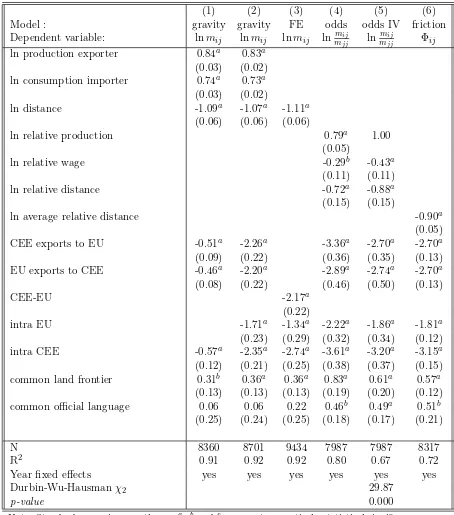
I estimate border effects for total manufactured bilateral imports of fifteen EU countries and twelve Central and East European countries with pooled ordinary least squares and year fixed effects and report results in table 1. Standard deviations are obtained with a robust clustering technique that allows error terms for the same country pair to be correlated. This permits to control at least partially for autocorrelation in the data. All coefficients have the expected sign and most of them are statistically significant. Production and consumption coefficients are close to unity and the distance elasticity of trade is not very different from -1, similar to most empirical studies in the literature. The parameters of interest are the coefficients on group (trade type) dichotomic variables. The fist column shows estimates of international trade costs relative to intra-EU costs. Negative coefficients of group dummies indicate that intra-EU trade is subject to lowest trade costs, justifying its use as reference for other European trade flows. A core EU country exports on average

37% [= (1− exp(−0.46)) × 100] less to a NMS than to another EU country, imports

40% [= (1−exp(−0.51))×100] less from a NMS than from a EU partner, and two NMS trade 43% [= (1−exp(−0.57))×100] less than two core EU countries equally large and distant. Border effect estimates obtained with equation (21) are presented in column 2. Setting all group variables equal to zero yields an estimation of domestic trade and trade costs for each type of international trade flows are obtained relative to this reference level. Thus, intra-EU border effects or trade costs are5.5 [= exp(1.71)]times larger than domestic trade costs; EU exports to and imports from NMS are 9.0 [= exp(2.20)] and respectively

9.6 [= exp(2.26)] times more expensive than trading within national borders. Trade costs between NMS from Central and Eastern Europe are the largest: 10.5 [= exp(2.35)] times domestic costs. Hence, both CEE-EU and intra-CEE trade integration lies bellow the level reached by the fifteen core-EU members.

The positive and significant coefficient on the common land border variable confirms the intuition that neighbor countries trade more with each other. This can be due to lower trade costs between these countries, as well as to more similar consumer preferences. The non significant coefficient of the common language dummy is due to its high correlation with the common border variable, the low number of dyads sharing both characteristics in the sample, and their uneven distribution across country groups.6

Including internal trade in estimations (column 2) keeps the coefficients on all variables almost unchanged (relative to column 1), and sets forward the fact that both EU and CEE countries rely much more on domestic than foreign partners.

Border effects of similar magnitude of are obtained with the other three trade specifi-cations. Thefixed-effects model (column 3) estimates that a EU member country buys on average about3.8 [= exp(1.34)]times more from itself than from another EU country, while a similar NMS buys about 15.5 [= exp(2.74)] times more. Trade between EU and NMS is less than half of the intra-EU trade, when controlling for market and supply capacities, distance and common language and land border.

6

Table 1: European trade integration: total manufactured imports

(1) (2) (3) (4) (5) (6) Model : gravity gravity FE odds odds IV friction Dependent variable: lnmij lnmij lnmij lnm_mij_jj lnm_mjjij Φij lnproduction exporter 0.84a 0.83a

(0.03) (0.02)

lnconsumption importer 0.74a _0.73a

(0.03) (0.02)

lndistance -1.09a -1.07a -1.11a (0.06) (0.06) (0.06)

lnrelative production 0.79a 1.00 (0.05)

lnrelative wage -0.29b _-0.43a

(0.11) (0.11)

lnrelative distance -0.72a -0.88a (0.15) (0.15)

lnaverage relative distance -0.90a (0.05) CEE exports to EU -0.51a _-2.26a _-3.36a _-2.70a _-2.70a

(0.09) (0.22) (0.36) (0.35) (0.13) EU exports to CEE -0.46a -2.20a -2.89a -2.74a -2.70a (0.08) (0.22) (0.46) (0.50) (0.13)

CEE-EU -2.17a

(0.22)

intra EU -1.71a _-1.34a _-2.22a _-1.86a _-1.81a

(0.23) (0.29) (0.32) (0.34) (0.12) intra CEE -0.57a -2.35a -2.74a -3.61a -3.20a -3.15a (0.12) (0.21) (0.25) (0.38) (0.37) (0.15) common land frontier 0.31b _0.36a _0.36a _0.83a _0.61a _0.57a

(0.13) (0.13) (0.13) (0.19) (0.20) (0.12) common official language 0.06 0.06 0.22 0.46b _0.49a _0.51b

(0.25) (0.24) (0.25) (0.18) (0.17) (0.21)

N 8360 8701 9434 7987 7987 8317 R2

0.91 0.92 0.92 0.80 0.67 0.72 Year fixed effects yes yes yes yes yes yes Durbin-Wu-Hausman χ2 29.87

p-value 0.000

Note: Standard errors in parentheses: a_,b _andc _{represent respectively statistical significance} at the 1%, 5% and 10% levels.

on relative production, in line with the theoretical model, and use per capita GDP, em-ployment levels (size of labor force), and productivity as instruments for wages. Standard errors take into account the correlation of the error terms for a given importer. This is required by the specific form of the explained variable: the logarithm of the ratio between a imports from a foreign source and domestic purchases. All estimates are statistically significant at the 5% level. The low absolute value of the wage coefficient is due to the fact that wages reflect quite poorly product prices.7

I obtain larger absolute values for wage and distance coefficients when I correct the endogeneity bias. The use of instrumental variables (IV) also induces a drop in European border effects, which approach the estimates of the

fixed-effects model. Column 4 results confirm the relationship between CEE-EU trade costs in both directions established in columns 1 and 2: It costs less for EU countries to export to CEE partners than for NMS from Central and Eastern Europe to export to old EU. This difference vanishes with a IV estimator: CEE-EU trade in either direction is about fifteen times more expensive than trade with a domestic partner. Core EU countries with no common border or language trade with each other six times more than with themselves. More similar tastes and/or larger transaction costs lead to a higher border effect estimate for intra-CEE trade: 24.5 [= exp(3.20)].

The last column of table 1 displays the estimates of thefriction specification. Bilateral variables used to express trade costs are the only explanatory variables in this model. By construction, error terms are not independent across observations, but are assumed independent across importer-exporter couples. Estimates of border effects are very similar to the ones in column 5. The last three columns also show an enhanced effect of the common land border and confirm that countries that speak the same language face lower trade costs. As expected, theodds andfriction specifications generate larger border effects than thefixed-effects and standard gravity models. This difference is explained by the fact that in thefixed-effects approach importer and exporter dummies capture country-specific trade costs as well as some of the variance in consumer preferences, while in the odds and

friction specifications they are attributed to border effects. Therefore, if one believes that country-specific trade costs have are uniformly distributed and consumer preferences are highly uneven, one should rely on estimates in column 3. Estimates from columns 5 and 6 should be preferred in the opposite case. To summarize, depending on the specification, CEE-EU trade is on average 9 to 15 times inferior to domestic trade when keeping supply, demand, and trade costs constant. This ratio is 2.4 times larger than for trade between the old EU countries, but represents less than two-thirds of the similar ratio for intra-CEE trade.

Border effect estimates obtained with industry level data are shown in table 2.8

When trade is broken down by industries, an important number of zero value trade flows is observed. The problem with nil trade flows is that they do not occur randomly, but are the outcome of a selection procedure, e.g. a low supply or demand for a particular group of products. To correct for this sample self-selection bias I give a positive weight to the zero trade mass and employ a two-stage Heckman estimator: a first-stage probit model and a second-stage pooled OLS model with year fixed effects. A statistically significant

7

In reality the labor is not the unique factor of production and there are many additional distortions in the price structure not captured by the model.

8

Table 2: European trade integration: border effects with industry-level data

Country pairs that do not share a common land border and do not speak the same language

Trade flows gravity FE odds odds IV friction CEE exports to EU 11.3 15.8 27.4 15.7 18.9 EU exoprts to CEE 10.1 15.8 11.2 7.6 18.9 Intra EU trade 3.8 6.4 6.6 4.2 6.6 Intra CEE trade 21.0 23.9 27.6 17.4 29.0

Country pairs that share a common land border and speak the same language

Trade flows gravity FE odds odds IV friction CEE exports to EU 6.0 6.5 7.7 5.5 6.5 EU exports to CEE 5.4 6.5 3.2 2.7 6.5 Intra EU trade 2.0 2.6 1.9 1.5 2.2 Intra CEE trade 11.2 9.8 7.8 6.1 10.0

Note: Border effects are computed using estimated coefficients of equations (21), (22), (23) and (24) for each year with industry level data. Effects for countries with no common land border or language are represented.

coefficient of Mills’ ratio in the second stage is obtained for the fixed-effects and odds

specifications, indicating the necessity of this adjustment. Compared to the results for the aggregate manufactured sector, estimated coefficients are slightly lower for supply and demand variables but larger in absolute terms for distance and common land border. The positive and significant pro-trade effect of a common language spoken by the exporter and the importer appears in all the three specifications compatible with the theoretical model. Estimated border effects for all trade types and all specifications except the odds are larger when industry level data are employed. This finding testifies that most European trade liberalization was concentrated in a small number of large size industries. The use of aggregate manufacturing data underestimates the amount of ‘missing’ international trade because it disproportionately reflects large sectors with low barriers to trade. Lower border effects with industry level data and the odds specification are due to the larger selection bias. The odds specification uses domestic trade of the same importing country and in the same industry as reference for international flows. Differently, in gravity and fixed-effects models domestic trade of any country in the sample and any sector may serve as reference after controlling for market supply, demand and trade costs. Therefore, industry level border effects obtained with theodds method are more accurate. The preference over results with the friction model is due to the fact that the odds specification allows for different border effects for CEE exports to core EU and CEE imports from EU.

to EU face higher trade barriers than flows in the opposite direction. This counterintuitive result is robust to changes in the estimation procedure or country panel. The apparent paradox can be explained by the fact that EU countries liberalized first their domestic markets for small and medium size industries, and kept until late 1990s relatively important barriers in several key CEE industries such as textiles and food products, while CEE countries have adopted a distinct policy towards EU partners.

4

Trade Potential and East-West European Integration

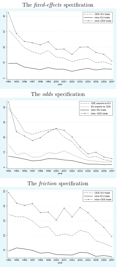
The important steps undertaken by Eastern and Western European countries for the re-moval of politically imposed distortions on bilateral exchanges at the beginning of 1990s, as well as efforts engaged with the scheduled EU enlargement translated into a continuous increase in trade between these countries. The drop in European cross-border trade costs is well pictured by the evolution on regional border effects. Figure 1 show that border effects for both CEE-EU and intra-EU trade reduced considerably from 1994 to 2007. This conclusion is reached regardless of the trade specification employed. Theodds specification suggests that by the end of the period intra-EU trade costs were less than twice the level of costs for domestic trade, while intra-CEE and CEE-EU trade costs where respectively six and four times larger than this reference level. The reduction of trade costs continued even after CEE countries integrated the European Union.

While strengthening trade between old and new members, EU enlargement affected as well trade between NMS. According to the literature (Maurel, 1998, Gros and Gon-ciarz, 1996, Baldwin, 1993, Nilson, 2000), the reintegration of CEE countries into the world economy in the early 1990s was accompanied by their disengagement from intra-CEE integration. The decline of trade with other intra-CEE partners was beyond its normal level, pointing out the strong competition between former socialist economies for obtaining a higher share of the larger and more attractive core-EU market, and for increasing their chances for accession. With most of CEE countries joining the union, this rivalry has been significantly reduced, and intra-CEE trade has regained attraction. Indeed, as shown in figure 1, intra-CEE border effects dropped by over thirty points from 1994 to 2007.

The reintegration of Central and Eastern European countries in the world economy after the collapse of the communist system was accompanied by the reorientation of their foreign trade towards the European Union. The important drop in CEE-EU border effects in figure 1, especially for CEE exports to core EU countries, reflects this reinforcement of regional integration in Europe.

Figure 1: European trade integration: border effects

The fixed-effects specification

0

10

20

30

40

1994 1995 1996 1997 1998 1999 2000 2001 2002 2003 2004 2005 2006 2007 year

CEE−EU trade intra−EU trade intra−CEE trade

The odds specification

0

10

20

30

40

1994 1995 1996 1997 1998 1999 2000 2001 2002 2003 2004 2005 2006 2007 year

CEE exports to EU EU exports to CEE intra−EU trade intra−CEE trade

The friction specification

10

20

30

40

50

1994 1995 1996 1997 1998 1999 2000 2001 2002 2003 2004 2005 2006 2007 year

CEE−EU trade intra−EU trade intra−CEE trade

costs associated with each trade type to intra-EU costs. I define the potential of CEE-EU and intra-EU trade as the ratio of the corresponding border effects:

CEE-EU trade potential = CEE-EU border effect

intra-EU border effect, (25)

intra-CEE trade potential= intra-CEE border effect

intra-EU border effect . (26) Trade potentials obtained in this way reflect a trade integration in terms of border effects. This kind of integration reaches its peak when the two groups of countries have identical cross-border trade costs and preferences. I compute trade potentials using equa-tions (25) and (26) and border effect estimates obtained with each of the four trade spec-ifications employed in section 3. Whenever possible, separate border effects for each type of trade (CEE exports to and imports from the EU, and intra-CEE trade) are computed. Average East-West European trade potential for flows in both directions are estimated using a single dummy for CEE-EU trade.

For comparison, I also compute trade potentials using the traditional methods employed in the literature and display the results in table 3. For comparability, I use again trade flows between the old EU countries as reference. Unlike the border effect ratio method presented above, traditional trade potential models rely exclusively on cross-border flows. Therefore I estimate equation (21) on the sub-panel of international trade and use the resulting coefficients to compare CEE-EU and respectively intra-EU trade with the level of intra-EU trade. A fist method, that I call gravity 1, consists in expressing CEE-EU and intra-EU trade flows as percentage of intra-EU flows and attribute the difference up to 100% to the trade potential. Alternatively, gravity 2 computes trade potentials as the difference between the level of trade predicted by equation (21) and actual trade. Finally, in line with the literature on trade potential,9

withgravity 3 I estimate (21) for trade of the reference group, intra-EU trade in our case and use obtained coefficients along with data on production, consumption, bilateral distance, and bilateral linkages (common language and land border) to predict the ‘normal’ level of trade for the rest of flows. The difference between actual and predicted (or ‘normal’) trade levels gives the potential of trade. Results with all three methods for the first and last year in the panel are displayed in the upper part of table 3. Trade potentials obtained with the innovative approach introduced in this paper are shown in the last part of table 3. The four rows correspond to the different trade specifications used to estimate European border effects.

A first conclusion that stems from table 3 is that traditional methods employed in the literature, gravity 1, gravity 2 and gravity 3, yield small trade potentials. For all types of trade flows these values are considerably lower than trade potentials obtained with the border effects ratio method. Thus, traditional methods overestimate the level of trade integration in the region. For exampl, according togravity 1, in 1994 CEE-EU trade represented only 12% of the level of intra-EU trade for comparable countries, corresponding to a trade potential of 88%. Meanwhile, the ratio of border effects produces a trade potential four times larger. Gravity2 andgravity 3 find small and non-significant variations

9

Table 3: European Trade Potential (in % of actual trade)

Type of trade flows

Method CEE to EU EU to CEE CEE-EU intra-CEE 1994 2007 1994 2007 1994 2007 1994 2007 Traditional trade potential models with international trade flows only

gravity 1 ∗ _{78 64 76 50 77 58 88 77}

gravity 2 † 44 48 52 56 48 52 51 52

gravity 3 ‡ _{45 44 53 52 49 48 50 48}

Border effects ratio method: equations (25) and (26)

McCallum (1995) gravity 420 253 399 192 409 221 735 388

fixed-effects specification 334 152 449 191

odds specification 535 232 204 186 335 209 590 314

friction specification 362 219 520 339

Note: Trade potentials are computed with industry level data: ∗ _{as exponential values of estimated group dummies;} † _{as the difference between actual and normal trade;}

‡ _{as the difference between actual and normal trade, using intra-EU trade as reference.}

in the CEE-EU and intra-CEE trade integration from 1994 to 2007. With trade potentials computed as the difference between gravity-predicted (‘normal’) and actual volumes of trade, flows between old and new member states and flows within the NMS group in any year during this period are estimated at found to be only 50% under their potential level. In addition, these models predict slightly larger trade barriers for EU exports to CEE countries than for flows in the opposite direction, a finding contrary to results obtained with the other approaches.

When GDP and population data are used instead of industry-level production and con-sumption in equation (21), a simplification frequently adopted in the traditional literature, trade potentials predicted by traditional models are even lower (results not displayed). With these adjustments I find that East-West trade integration, if present, was very slow or only marginal. In half of the cases the trade potential for CEE-EU flows increased over the studied period, which comes at odds with the evolution of the regions’ economic and political environment. As for intra-CEE trade, this approach does not predict a increased regional integration, but rather a growing reticence of CEE countries to exchange mutually. The new method for measuring trade potentials introduced above produces similar val-ues with border effects estimated by fixed-effects, odds and friction specifications. This approach situates East-West trade potential in 2007 between 152% and 219%. Depending on the trade specification, during the considered period CEE-EU trade regained between 35% and 48% of its 1994 potential. The odds specification is the only to produce differ-entiated results by flows’ direction. For all years in the sample the model exhibits CEE exports to EU more distant from their potential than opposite flows. This matches the finding pf lower access of products from Eastern Europe to Western EU markets from the previous section.

1990s. In 1994 regional intra-CEE trade amounted to 15-18% of its potential level. Re-gardless of the border effects estimates used to compute trade potentials in table 3, I find an important increase of the intra-CEE integration. This reflects the drastic reorientation of foreign trade of these countries in the first years following the collapse of the socialist system. Advances in the process of transition and the development of regional economic agreements (CEFTA, the Free Trade Agreement of Baltic states) encouraged regional trade, which augmented enormously in terms of its potential. Lower trade potentials under the

fixed-effects specification, compared to odds and friction specifications, are caused by im-portant country specific trade costs encountered by CEE partners (e.g. poor institutions or transport systems) captured by country dummies.

One can also note that using a specification compatible with trade theory is also impor-tant. Indeed, considerably larger trade potentials are obtained when one uses border effects estimated with traditional gravity: over 700% for intra-CEE trade with McCallum (1995) gravity compared to only 450% with thefixed-effects specification. This difference in results reminds that atheoretical models are subject to non-negligible biases.

The large difference in trade potentials between the upper and lower part of table 3 comes from the use of different criteria for evaluating trade integration. Traditional trade potential models ignore domestic trade and assign ‘normal’ trade to the prediction of the gravity equation. The method introduced in this paper compares directly trade costs arising in East-West European and intra-CEE transactions to costs existing between EU trade partners. Trade within the domestic market is used as benchmark for the very estimation of these costs. Thus, our method accounts for the discrepancy between domestic and cross-border trade integration. It is important to signal that not all ‘missing’ international trade is attributed to the trade potential, but only the proportion which corresponds to the difference in trade impediments for specific types of flows. Regional integration is evaluated here in terms of trade costs, expected to converge to the lower intra-EU level. This uniformization of costs will result in increased trade with more distant partners and weaker concentration of trade in the immediate neighborhood.

Larger potentials obtained with the new method confirm the necessity to account for domestic trade in predicting the trade creation effects of regional integration. The dis-regard of internal trade opportunities is likely to largely underestimate trade potentials. Our method has the advantage of accounting for total international barriers to trade and therefore produces results more in compliance with integration efforts made by countries. Globally, the access of CEE goods to the old EU markets improved considerably during from 1994 to 2007, and a large part of the potential European trade creation was already accomplished. Nevertheless, by the year 2007 the left CEE-EU trade potential was signifi-cantly larger than actual trade, implying more than a twofold possible increase of trade in the years to follow.

In table 4 of the Appendix A I show industry-level effects on trade of European integra-tion with thefixed-effects, odds and friction specifications.10

The first six columns refer to trade potentials in 1994, and the last six for the year 2007. The first thing to notice is that with a few exceptions trade creation effects are observed for all industries, both CEE-EU and intra-EU trade, and under all specifications. The largest trade creation for both

two-10

way East-West European trade and intra-CEE trade was observed for rubber products and electrical machinery. Non-electrical machinery and iron and steel products also enjoyed im-portant trade creation. Trade between NMS increased largely in industrial chemicals and textiles. The lowest trade integration is found in the tobacco industry, subject to specific domestic regulations especially in core EU countries. In the case of intra-CEE trade, how-ever, this is due to the fact that trade in tobacco production between CEE countries was below its potential level even in 1994. For other chemical products and wearing apparel European trade has even lost some of its potential. This can be explained by the increased competition in these industries with products from emerging Asian countries and in partic-ular China. Moderate effects on trade are obtained for the rest of industries. By the year 2007 CEE-EU trade remains largely inferior to its potential (less than one third) only in seven: food products, beverages, tobacco, chemicals, iron and steel industries, professional and scientific and measuring and controlling equipment, leather products and printing and publishing. As expected, their number is larger for intra-CEE trade.

The reduction of both trade barriers and trade potentials for CEE-EU trade coincided with an even more impressive evolution for trade between NMS. These results disseminate the fears formulated by politicians and some authors that that CEE-EU trade integration will be accompanied by a lower commitment of CEE countries to regional integration, reflected by larger intra-CEE border effects and trade potentials at the beginning of the period. Still, figures in table 3 show that manufactured trade between CEE countries may expand to as much as two to three times the actual volume.

5

Conclusions

Trade both between CEE and between CEE and EU countries improved remarkably during the last two decades, both in terms of border effects and trade potentials. The paper shows that there is still place for important growth in bilateral CEE-EU transactions. This result contradicts with most trade potential gravity models that claim that East-West European trade has already reached its highest integration level. Much higher trade potentials for both CEE-EU and intra-CEE trade are obtained when one controls for the amount of trade within national borders. Results are very robust and are confirmed by three different theoretically compatible trade specifications used. Thus, at the beginning of the twenty-first century trade between CEE and EU countries represented less than half of its attainable level, suggesting a possible 150% to 200% increase with further EU integration. As for trade between NMS, its potential ranges depending on the model between 190% and 340%, despite the strong reduction of bilateral border effects between these countries achieved during the 1990s.

References

Armington, P. (1969). A theory of demand for products distinguished by place of produc-tion. IMF Staff Papers (16), 159–176.

Aymo Brunetti, G. K. and B. Weder (1997). Institutional obstacles for doing business.

World Bank Research Paper.

Baldwin, R. (1993). The potential for trade between the countries of efta and central and eastern europe. CEPR discussion Paper (853).

Bergsrand, J. H. (1989). The generalized gravity equation, monopolistic competition, and the evolution of the factor-proportions theory. Review of Economics and Statistics 23, 143–153.

Combes, P.-P., M. Lafourcade, and T. Mayer (2005). The trade creating effects of business and social networks: Evidence from France. Journal of International Economics 66(1), 1–29.

Deardorff, A. V. (1998). The Regionalization of the World Economy (University of Chicago Press ed.)., Chapter Determinants of Bilateral Trade: Does Gravity Work in a Neoclas-sical World?, pp. 7–28. NBER. Jeffrey A. Frankel.

Dixit, A. and J. Stiglitz (1977). Monopolistic competition and optimum product diversity.

American Economic Review 67(3), 297–308.

Fontagne, Lionel, M. F. and M. Pajot (1999). Le potential d’échanges entre l’union eu-ropéenne et les peco. Revue Economique 50(6), 1139–1168.

Gros, D. and A. Gonciarz (1996). A note on the trading potential of central and eastern europe. European Journal of Political Economy 12(4), 709–721.

Hamilton, C. and L. A. Winters (1992). Opening up international trade with eastern europe. Economic Policy 14, 77–116.

Head, K. and T. Mayer (2000). Non-europe: The magnitude and causes of market frag-mentation in europe. Weltwirtschaftliches Archiv 136(2), 285–314.

Head, K. and J. Ries (2001). Increasing returns versus national product differentiation as an explanation for the pattern of us-canada trade. American Economic Review 91(4), 858–876.

Krugman, P. (1980). Scale economies, product differentiation, and the pattern of trade.

American Economic Review 70(5), 950–959.

Maurel, M. and G. Cheikbossian (1998). The new geography of eastern european trade.

Kyklos 51(1), 45–72.

Nilsson, L. (2000). Trade integration and the eu economic membership criteria. European Journal of Political Economy 16(4), 807–827.

Papazoglou, C., E. J. Pentecost, and H. Marques (2006, 08). A gravity model forecast of the potential trade effects of eu enlargement: Lessons from 2004 and path-dependency in integration. The World Economy 29(8), 1077–1089.

Rauch, J. E. (2001). Business and social networks in international trade. Journal of Economic Literature 39(4), 1177–1203.

Redding, S. and A. J. Venables (2004). Economic geography and international inequality.

Journal of International Economics 62, 53–82.

Rose, A. and E. van Wincoop (2001). National money as a barrier to international trade: The real case for currency union. American Economic Review.

Wang, Z. K. and L. Winters (1991). The trading potential of eastern europe. CEPR Discussion Paper (610).

Wei, S.-J. (1996). Intranational versus international trade: How stubborn are nations in global integration. NBER Working Paper (5531).

A

Data and additional results

The empirical application of theoretically derived trade equations encounters both data availability and comparability problems. The use of different classifications, definitions and registration criteria even for such standard economic variables as production and trade may represent an additional source of errors and biases in results. The latter are yet more pronounced in the estimation of border effects when internal trade volumes are computed as the difference between national production and total exports in absence of regional data. The present study carries over a sample of 27 countries: fifteen core EU members with Belgium and Luxembourg aggregated under a single observation, and twelve Central and East European countries, and a fourteen-year period from 1994 to 2007. Of the twelve CEE countries of the panel ten have joined the EU in May 2004 and two in January 2007. Two levels of aggregation are considered: total manufacturing industry, and 26 product industries according to the ISIC Rev.2 classification.

Cheptea

Bo

rder

Effects

and

Europ

ean

Integration

Industry CEE-EU trade Intra-CEE trade

FE odds friction FE odds friction FE odds friction FE odds friction

1994 1994 1994 2007 2007 2007 1994 1994 1994 2007 2007 2007

Food 411 469 461 257 320 316 402 799 592 365 448 436

Beverage 876 652 891 518 786 810 980 673 929 530 837 963

Tobacco 106 98 124 1371 2145 1778 63 23 30 3993 719 852

Textiles 335 294 373 92 98 101 597 1058 995 193 185 154

Wearing apparel, except footwear 76 106 163 81 275 171 62 255 497 132 1524 686

Leather 314 272 235 127 369 675 807 1064 959 175 1124 823

Footwear 169 156 143 59 149 138 223 327 257 27 905 387

Wood, except furniture 234 296 297 118 105 104 257 466 402 153 120 122

Furniture 303 438 457 105 123 126 1011 115 905 271 284 276

Paper and paper products 437 412 441 139 177 174 321 372 311 112 140 131

Printing and publishing 469 653 441 202 273 272 440 657 349 358 514 511

Industrial chemicals 385 356 418 169 191 188 410 298 479 123 108 122

Other chemical products 433 438 368 451 431 584 180 726 333 511 288 669

Rubber products 500 567 509 87 117 112 764 1230 1229 77 115 80

Plastic products 451 378 488 202 224 216 574 604 817 394 429 410

Pottery, china and earthenware 444 395 488 183 217 222 1153 989 1956 233 346 275

Glass and glass products 449 485 457 138 148 134 554 1029 770 230 228 199

Other non-metallic mineral products 403 323 337 164 253 250 606 532 477 157 301 252

Iron and steel basic industries 1216 1349 1111 263 229 231 3260 3588 1822 429 196 307

Non-ferrous metal basic industries 572 637 696 182 224 163 855 602 578 224 198 162

Fabricated metal products 209 220 207 69 75 78 340 632 431 87 112 116

Machinery except electrical 347 428 392 132 134 138 473 972 707 199 136 253

Electrical machinery and appliances 412 322 387 71 86 83 928 862 723 81 98 72

Transport equipment 696 399 610 141 171 144 899 959 943 213 176 115

Professional, scientific, measuring, and controlling equipment, photographic and optical goods

497 765 664 263 242 279 871 1748 909 811 509 867

Other manufacturing 410 376 395 97 122 102 802 1702 1333 136 108 105