http://www.scirp.org/journal/ojs ISSN Online: 2161-7198
ISSN Print: 2161-718X
Comparison of REML and MINQUE for Estimated
Variance Components and Predicted Random
Effects
Nan Nan1, Johnie N. Jenkins2, Jack C. McCarty2, Jixiang Wu3*
1Department of Mathematics and Statistics; South Dakota State University, Brookings, SD, USA 2Crop Science Research Laboratory USDA-ARS, Mississippi State, MS, USA
3Agronomy, Horticulture, and Plant Science Department, South Dakota State University, Brookings, SD, USA
Abstract
Linear mixed model (LMM) approaches have been widely applied in many areas of research data analysis because they offer great flexibility for different data structures and linear model systems. In this study, emphasis is placed on comparing the prop-erties of two LMM approaches: restricted maximum likelihood (REML) and mini-mum norm quadratic unbiased estimation (MINQUE) with and without resampling techniques being included. Bias, testing power, Type I error, and computing time were compared between REML and MINQUE approaches with and without Jack-knife technique based on 500 simulated data sets. Results showed that MINQUE and REML methods performed equally regarding bias, Type I error, and power. Jackknife- based MINQUE and REML greatly improved power compared to non-Jackknife based linear mixed model approaches. Results also showed that MINQUE is more time- saving compared to REML, especially with the use of resampling techniques and large data set analysis. Results from the actual cotton data analysis were in agreement with our simulated results. Therefore, Jackknife-based MINQUE approaches could be recommended to achieve desirable power with reduced time for a large data anal-ysis and model simulations.
Keywords
Linear Mixed Model Approaches, MINQUE, REML, Jackknife
1. Introduction
Linear mixed models (LMM) are a generalization of various linear models covering simple linear regression models, ANOVA models, and complex genetic models. LMM How to cite this paper: Nan, N., Jenkins,
J.N., McCarty, J.C. and Wu, J.X. (2016) Comparison of REML and MINQUE for Estimated Variance Components and Pre-dicted Random Effects. Open Journal of Statistics, 6, 814-823.
http://dx.doi.org/10.4236/ojs.2016.65067
Received: August 20, 2016 Accepted: October 15, 2016 Published: October 18, 2016
Copyright © 2016 by authors and Scientific Research Publishing Inc. This work is licensed under the Creative Commons Attribution International License (CC BY 4.0).
approaches including maximum likelihood (ML) [1], restricted maximum likelihood (REML) [2], and minimum norm quadratic unbiased estimation (MINQUE) [3] are among the most commonly used ones for variance component estimation and random effect prediction. Numerical comparisons of the statistical properties among these LMM approaches could help users choose appropriate approaches for various data analyses.
ML and REML approaches have been integrated into SAS [4] and into R such as lme4 [5][6] and ASReml [7]. Due to their popularity and long-term availability, a wide range of applications in various areas, has occurred. For example, based on a recent google scholar search in May, 2016, more than 43,000 publications were available. Both ML and REML approaches are based on the assumption that data are normally distri-buted (Laird and Ware, 1982) and require iterations [8]. Compared to ML and REML, MINQUE approaches were less popular. However, MINQUE approaches do not re-quire normally distributed data nor iterations [3][9]. Thus, they could offer more flex-ibility with reduced computational intensity. Since 1989, MINQUE approaches have been widely used in quantitative genetics studies [10]-[19].
Though LMM approaches are currently widely used, a potential issue associated with LMM is low power in statistical tests for variance components and random effects. With the use of jackknife methods, statistical powers could be significantly improved [20]-[22]. On the other hand, with resampling techniques, it is possible to generalize statistical tests for various parameters of interest. Resampling techniques including jackknife and permutation methods have been integrated in linear mixed model ap-proaches and two R packages, minque and qgtools, which are currently available online [23][24].
The aim of this study was to compare statistical properties between REML and MINQUE approaches with and without a jackknife technique [25] through Monte Carlo simulations. A cotton data set [25] including 24 genotypes under two environ-ments was used for both simulations and actual data analyses. These methods were compared regarding statistical power, Type I error, and computational time. Results in-cluding variance components and genotypic effects from actual data analysis were also compared. Results could provide statistical information on appropriate use of these LMM approaches.
2. Materials and Methods
2.1. Materials
used for our actual data analysis. The data set, cot, is currently available in the R pack-age, minque [23].
2.2. Statistical Model and Methods
Given the data structure, the observation yijk standing for the genotype j under the kth
block in the environment i can be expressed by using the following linear mixed model: ( )
ijk i j ij k i ijk
y = +µ E +G +GE +B +e (1)
where Ei is an environmental effect and treated as fixed effect; Gj is a genotypic
ef-fect and treated as random; GEij is a genotype-by-environment interaction effect and
random; Bk i( ) is a random block effect within environment; and eijk is the random
error.
Two linear mixed model approaches, MINQUE and REML [2][3][9], were applied. In addition, a randomized 10-fold Jackknife technique [21] was integrated with these two linear mixed model approaches. Therefore, four combinations of methods in total were used for both simulation and actual data analysis. To simplify our description, we defined these four combinations of methods as: M1 = MINQUE without jackknife; M2 = REML without jackknife; M3 = MINQUE with jackknife; and M4 = REML with jackknife. Regarding simulation studies, there could be numerous parameter settings, however, we only considered two representative parameter settings because the major aim of this study was to compare statistical properties among these four methods. The first setting was to preset all variance components to 20 (interested users may use other settings), targeting power and bias. The second setting was to preset all variance com-ponents to zero except the random error variance which was 20, targeting Type I error and bias for all variance components except random error variance. For each parameter setting, five hundred simulated data sets [26][27] were generated and analyzed by each combination of these four methods. Statistical properties including bias, and testing power/Type I error were calculated for each method [28][29]. Type I error is the false significance rate for a preset variance component being zero while testing power is the true significance rate for a positive preset variance component over 500 simulations. The bias is for each variance component is the deviation of mean estimated variance component from the preset variance component (0 or 20 in this study) which is given by Equation (2):
0
ˆ
Bias= −θ θ (2)
where, θ0 is a preset variance component and θˆ is mean estimated variance
com-ponent. We briefly defined the following terms. The standard error (SE) is defined by
( )
ˆSE θ , a standard error for a mean estimated variance component. In addition, com-putational time (in seconds) was recorded for every 100 simulations out of 500 simula-tions (Table 3).
functions that are available in the R package minque [23] under the R Studio environ-ment [31]. The computational time recorded for simulation was based on HP Z440 with 32G ram under Windows 7 64-bit operation system.
3. Results and Discussion
3.1. Simulation Results
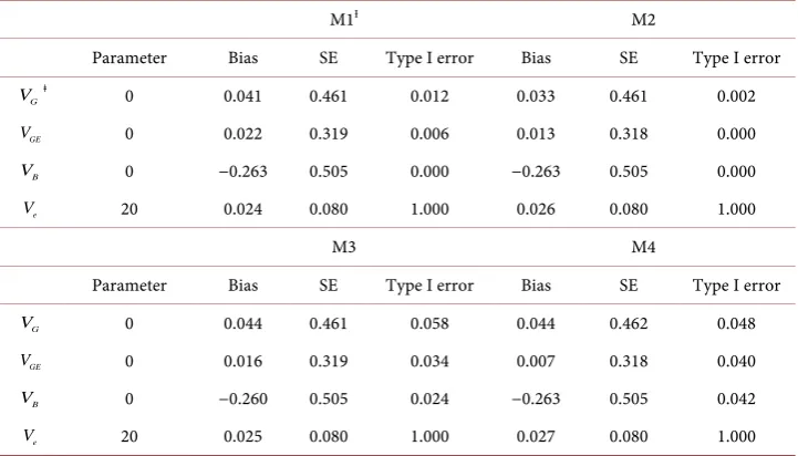
Bias, standard error, power, Type I error, and computational time based on 500 simu-lated data for four methods are summarized in Table 1 and Table 2. Results showed that bias for each variance component was similar among the four methods (M1-M4) (Table 1 and Table 2). Standard errors (SE) for each variance component among 500 estimates were also similar for the four methods (Table 1 and Table 2). Non-Jackknife based MINQUE and REML methods (M1 and M2) had similar power (at the probabil-ity level of 5%). However, Jackknife based REML and MINQUE methods (M3 and M4) had improved power for variances of genotypic and block effects compared to non-Jackknife based methods(M1 and M2) (Table 1). All four methods yield acceptable Type I error (around 5% or lower) for all variance components except the random error variance component (Table 2). Overall, both MINQUE and REML performed equally well regarding bias, power, and Type I error for variance component estimation. How-ever, jackknife based MINQUE and REML could greatly improve power with accepta-ble Type I error compared to non-jackknife based methods.
Computational time in seconds used for each 100 simulations for each method and parameter setting is given in Table 3. Though other tasks were possible active during
Table 1. Estimated bias, standard error (SE), and power (at 0.05) for four preset components
based on 500 simulated data sets with four methods.
M1Ɨ M2
Parameter Bias SE Power Bias SE Power
G
V ǂ 20 0.041 0.461 0.664 0.033 0.461 0.666
GE
V 20 0.022 0.319 1.000 0.013 0.318 1.000
B
V 20 −0.263 0.505 0.786 −0.263 0.505 0.788
e
V 20 0.024 0.080 1.000 0.026 0.080 1.000
M3 M4
Parameter Bias SE Power Bias SE Power
G
V 20 0.044 0.461 0.944 0.044 0.462 0.934
GE
V 20 0.016 0.319 1.000 0.007 0.318 1.000
B
V 20 −0.260 0.505 0.998 −0.263 0.505 0.998
e
V 20 0.025 0.080 1.000 0.027 0.080 1.000
Ɨ: M1 = MINQUE approach without Jackknife; M2 = REML approach without Jackknife; M3 = MINQUE approach
with Jackknife; and M4 = REML approach with Jackknife ǂ:
G
V = variance component for genotype effects; VGE = variance component for genotype and environment
Table 2. Estimated bias, standard error (SE), and Type I error (at 0.05) for four preset compo-nents based on 500 simulated data sets with four methods.
M1Ɨ M2
Parameter Bias SE Type I error Bias SE Type I error
G
V ǂ 0 0.041 0.461 0.012 0.033 0.461 0.002
GE
V 0 0.022 0.319 0.006 0.013 0.318 0.000
B
V 0 −0.263 0.505 0.000 −0.263 0.505 0.000
e
V 20 0.024 0.080 1.000 0.026 0.080 1.000
M3 M4
Parameter Bias SE Type I error Bias SE Type I error
G
V 0 0.044 0.461 0.058 0.044 0.462 0.048
GE
V 0 0.016 0.319 0.034 0.007 0.318 0.040
B
V 0 −0.260 0.505 0.024 −0.263 0.505 0.042
e
V 20 0.025 0.080 1.000 0.027 0.080 1.000
Ɨ: M1 = MINQUE approach without Jackknife; M2 = REML approach without Jackknife; M3 = MINQUE approach
with Jackknife; and M4 = REML approach with Jackknife ǂ:
G
V =variance component for genotype effects; VGL = variance component for genotype and environment
inte-raction effects; VB = variance component for block effects; and Ve = variance component for random error.
Table 3. Computational time (seconds) recorded each 100 simulations out of 500 simulations for
each method and parameter setting.
Parameter setting 1Ɨ Parameter setting 2
M1ǂ M2 M3 M4 M1 M2 M3 M4
1st 100 14.8 17.6 18.4 157.8 10.7 20.7 10.6 189.6
2nd 100 13.0 15.9 18.1 153.6 10.8 20.6 10.7 188.4
3rd 100 13.1 16.0 18.1 154.2 10.7 19.5 10.3 184.2
4th 100 13.1 16.1 17.9 154.8 10.9 20.6 10.8 193.8
5th 100 12.9 15.9 18.5 154.2 10.8 21.2 11.6 198.6
Total 66.9 81.5 91.0 774.6 53.9 102.6 54.0 954.6
Ɨ: Parameter settings 1: all variance components were preset as 20; Parameter settings 2: all variance components
were preset as 0 except the error variance component being set to 20.
ǂ: M1 = MINQUE approach without Jackknife; M2 = REML approach without Jackknife; M3 = MINQUE approach
with Jackknife; and M4 = REML approach with Jackknife.
[image:5.595.195.554.398.529.2]for the parameter setting 2 compared to the parameter setting 1. Our repeated simula-tions showed the same pattern (results not shown). One possible reason is that REML may need more iterations to converge for zero or negative variance components than for positive variance components. M4 was over eight-fold slower compared to M3 for the parameter setting 1 while 17 times slower for the parameter setting 2. Therefore, the results showed that MINQUE approach with or with jackknife was very time-saving yet yielded almost identical results compared to REML approach especially integrated with resampling process.
3.2. Actual Data Analysis
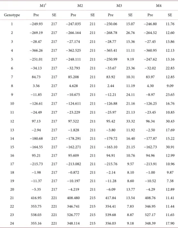
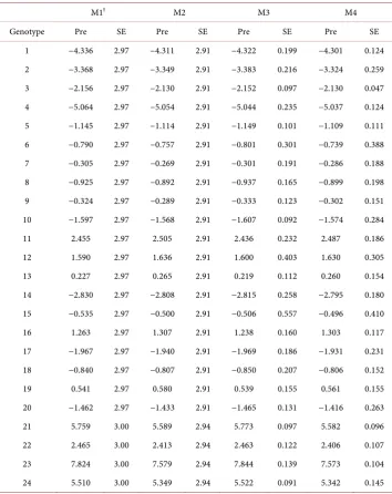
With the same model, two agronomic traits: cotton lint yield (LY) and lint percentage (LP), were analyzed by the same four methods used in our simulation studies. Esti-mated variance components for these two traits are summarized in Table 4 and Table 5 while predicted genotypic effects are presented in Table 6 and Table 7. Results showed that estimated variance components were similar for four methods for each of two traits while M3 and M4 yielded smaller standard error compared to M1 and M2 (Table 4 and Table 5). On the other hand, all four methods yielded similar predicted genotypic ef-fects while M3 and M4 had lower standard errors compared to M1 and M2 (Table 6 and Table 7). The results in Tables 4-7 showed that Jackknife technique integrated
Table 4. Estimated variance components for lint yield (LY) by four methods.
Parameter M1
Ɨ M2 M3 M4
Est SE Est SE Est SE Est SE
G
V 52,068 16,220 50,356 16,031 52,395 1567 50,548 1137
GL
V 333 1230 2379 2105 502 538 2322 681
B
V 838 890 848 890 803 324 806 335
e
V 25,168 2296 24,799 2275 25,312 888 24,904 833
Ɨ: M1 = MINQUE approach without Jackknife; M2 = REML approach without Jackknife; M3 = MINQUE approach
with Jackknife; and M4 = REML approach with Jackknife
ǂ:
G
V = variance component for genotype effects; VGL = variance component for genotype and location
interac-tion effects; VB = variance component for block effects; and Ve = variance component random error.
Table 5. Estimated variance components for lint percentage (LP) by four methods.
Parameter M1
Ɨ M2 M3 M4
Est SE Est SE Est SE Est SE
G
V 9.661 2.977 9.299 2.877 9.720 0.247 9.296 0.252
GL
V 0.460 0.242 0.509 0.260 0.513 0.276 0.537 0.176
B
V 0.129 0.103 0.128 0.103 0.132 0.036 0.128 0.016
e
V 1.798 0.166 1.805 0.166 1.774 0.159 1.790 0.085
Ɨ: M1 = MINQUE approach without Jackknife; M2 = REML approach without Jackknife; M3 = MINQUE approach with Jackknife; and M4 = REML approach with Jackknife
ǂ:
G
V = variance component for genotype effects; VGL = variance component for genotype and location
Table 6. Predicted genotypic effects for lint yield (LY, kg/ha) by four methods.
M1Ɨ M2 M3 M4
Genotype Pre SE Pre SE Pre SE Pre SE
1 −249.93 217 −247.035 211 −250.06 15.07 −246.80 11.76
2 −269.19 217 −266.164 211 −268.78 26.76 −264.52 12.60
3 −28.47 217 −27.174 211 −28.77 15.36 −27.45 13.86
4 −366.26 217 −362.525 211 −365.41 11.11 −360.95 12.13
5 −251.01 217 −248.111 211 −250.99 9.19 −247.62 13.16
6 −34.13 217 −32.793 211 −33.67 23.36 −32.02 22.83
7 84.73 217 85.208 211 83.92 10.31 83.97 12.85
8 3.56 217 4.628 211 2.44 11.19 4.30 9.09
9 −11.85 217 −10.675 211 −12.21 24.11 −8.97 23.65
10 −126.61 217 −124.611 211 −126.88 21.16 −126.25 16.76
11 −24.49 217 −23.229 211 −25.97 21.13 −23.45 10.85
12 97.13 217 97.522 211 95.42 33.32 96.34 30.43
13 −2.94 217 −1.828 211 −3.80 11.92 −2.50 17.69
14 −180.68 217 −178.291 211 −179.72 16.40 −177.87 15.22
15 −164.55 217 −162.271 211 −163.10 21.15 −162.73 30.91
16 95.21 217 95.609 211 94.91 10.76 94.96 12.99
17 −215.73 217 −213.082 211 −215.76 9.57 −213.91 10.96
18 −1.98 217 −0.872 211 −2.14 8.10 −1.00 9.87
19 −11.37 217 −10.197 211 −11.28 8.60 −10.52 7.38
20 −5.35 217 −4.219 211 −6.09 13.77 −4.29 12.89
21 416.95 221 408.480 215 417.84 13.54 408.76 11.41
22 353.75 221 346.741 215 354.41 7.83 346.95 11.44
23 538.03 221 526.777 215 539.68 8.87 527.17 11.65
24 355.16 221 348.114 215 356.03 9.18 348.39 17.90
Ɨ: M1 = MINQUE approach without Jackknife; M2 = REML approach without Jackknife; M3 = MINQUE approach
with Jackknife; and M4 = REML approach with Jackknife.
with two LMM approaches could significantly reduce standard errors for these esti-mated variance components and predicted effects and thus statistical power for these parameters increased considerably with the use of jackknife method, as shown in Table 1. The results from actual data analysis were highly consistent with the simulated results.
Table 7. Predicted genotypic effects for lint percentage (LP, %) by four methods.
M1Ɨ M2 M3 M4
Genotype Pre SE Pre SE Pre SE Pre SE
1 −4.336 2.97 −4.311 2.91 −4.322 0.199 −4.301 0.124
2 −3.368 2.97 −3.349 2.91 −3.383 0.216 −3.324 0.259
3 −2.156 2.97 −2.130 2.91 −2.152 0.097 −2.130 0.047
4 −5.064 2.97 −5.054 2.91 −5.044 0.235 −5.037 0.124
5 −1.145 2.97 −1.114 2.91 −1.149 0.101 −1.109 0.111
6 −0.790 2.97 −0.757 2.91 −0.801 0.301 −0.739 0.388
7 −0.305 2.97 −0.269 2.91 −0.301 0.191 −0.286 0.188
8 −0.925 2.97 −0.892 2.91 −0.937 0.165 −0.899 0.198
9 −0.324 2.97 −0.289 2.91 −0.333 0.123 −0.302 0.151
10 −1.597 2.97 −1.568 2.91 −1.607 0.092 −1.574 0.284
11 2.455 2.97 2.505 2.91 2.436 0.232 2.487 0.186
12 1.590 2.97 1.636 2.91 1.600 0.403 1.630 0.305
13 0.227 2.97 0.265 2.91 0.219 0.112 0.260 0.154
14 −2.830 2.97 −2.808 2.91 −2.815 0.258 −2.795 0.180
15 −0.535 2.97 −0.500 2.91 −0.506 0.557 −0.496 0.410
16 1.263 2.97 1.307 2.91 1.238 0.160 1.303 0.117
17 −1.967 2.97 −1.940 2.91 −1.969 0.186 −1.931 0.231
18 −0.840 2.97 −0.807 2.91 −0.850 0.207 −0.806 0.152
19 0.541 2.97 0.580 2.91 0.539 0.155 0.561 0.155
20 −1.462 2.97 −1.433 2.91 −1.465 0.131 −1.416 0.263
21 5.759 3.00 5.589 2.94 5.773 0.097 5.582 0.096
22 2.465 3.00 2.413 2.94 2.463 0.122 2.406 0.107
23 7.824 3.00 7.579 2.94 7.844 0.139 7.573 0.104
24 5.510 3.00 5.349 2.94 5.522 0.091 5.342 0.145
Ɨ: M1 = MINQUE approach without Jackknife; M2 = REML approach without Jackknife; M3 = MINQUE approach
with Jackknife; and M4 = REML approach with Jackknife.
References
[1] Hartley, H.O. and Rao, J.N.K. (1967) Maximum-Likelihood Estimation for the Mixed Analysis of Variance Model. Biometrika, 54, 93-108.
http://dx.doi.org/10.1093/biomet/54.1-2.93
[2] Patterson, H.D. and Thompson, R. (1971) Recovery of Inter-Block Information When Block Size Are Unequal. Biometrika, 58, 545-554. http://dx.doi.org/10.1093/biomet/58.3.545
[3] Rao, C.R. (1971) Estimation of Variance and Covariance Components—MINQUE Theory.
Journal of Multivariate Analysis, 1, 257-275.
http://dx.doi.org/10.1016/0047-259X(71)90001-7
[4] Littell, R.C., et al. (2006) SAS for Mixed Models. SAS Institute Inc., Cary, NC.
[5] Bates, D., Mächler, M., Bolker, B. and Walker, S. (2015) Fitting Linear Mixed-Effects Models Using lme4. Journal of Statistical Software, 67, 1-48. http://dx.doi.org/10.18637/jss.v067.i01
[6] Demidenko, E. (2013) Mixed Models: Theory and Applications with R. John Wiley & Sons Inc., Hoboken.
[7] Butler, D., Cullis, B. and Gilmour, A. (2007) ASReml-R: An R Package for Mixed Models Using Residual Maximum Likelihood.
https://www.r-project.org/conferences/useR-2007/program/presentations/butler.pdf
[8] Searle, S.R., Casella, G. and McCulloch, C.E. (1992) Variance Components. Wiley, New York. http://dx.doi.org/10.1002/9780470316856
[9] Zhu, J. (1989) Estimation of Genetic Variance Components in the General Mixed Model. North Carolina State University, Raleigh, NC.
[10] Zhu, J. (1995) Analysis of Conditional Genetic-Effects and Variance-Components in Deve-lopmental Genetics. Genetics, 141, 1633-1639.
[11] McCarty, J.C., Jenkins, J.N., Tang, B. and Watson, C.E. (1996) Genetic Analysis of Primitive Cotton Germplasm Accessions. Crop Science, 36, 581-585.
http://dx.doi.org/10.2135/cropsci1996.0011183X003600030009x
[12] Tang, B., Jenkins, J.N., Watson, C.E., McCarty, J.C. and Creech, R.G. (1996) Evaluation of Genetic Variances, Heritabilities, and Correlations for Yield and Fiber Traits among Cotton F2 Hybrid Populations. Euphytica, 91, 315-322. http://dx.doi.org/10.1007/BF00033093 [13] Zhu, J. and Weir, B.S. (1996) Mixed Model Approaches for Diallel Analysis Based on a
Bio-Model. Genetics Research, 68, 233-240. http://dx.doi.org/10.1017/S0016672300034200
[14] Lou, X.Y. and Zhu, J. (2002) Analysis of Genetic Effects of Major Genes and Polygenes on Quantitative Traits. II. Genetic Models for Seed Traits of Crops. Theoretical and Applied Genetics, 105, 964-971. http://dx.doi.org/10.1007/s00122-002-0958-5
[15] McCarty, J.C., Jenkins, J.N. and Wu, J.X. (2004) Primitive Accession Derived Germplasm by Cultivar Crosses as Sources for Cotton Improvement: I. Phenotypic Values and Variance Components. Crop Science, 44, 1226-1230. http://dx.doi.org/10.2135/cropsci2004.1226
[16] Lou, X.Y. and Yang, M.C.K. (2006) Estimating Effects of a Single Gene and Polygenes on Quantitative Traits from a Diallel Design. Genetica, 128, 471-484.
http://dx.doi.org/10.1007/s10709-006-7853-y
[17] Wu, J., Xu, H. and Zhu, J. (1997) An Approach to Eliminating Systematic Errors in Genetic Analysis. International Conference on Mathematical Biology, Hangzhou, 26-29 May 1997, 265-270.
Components. Crop Science, 46, 1169-1178. http://dx.doi.org/10.2135/cropsci2005.08-0269
[19] Saha, S., Wu, J., Jenkins, J.N., McCarty, J.C. and Stelly, D.M. (2013) Interspecific Chromo-somal Effects on Agronomic Traits in Gossypium hirsutum by AD Analysis Using Inter-mated G. barbadense Chromosome Substitution Lines. Theoretical and Applied Genetics, 126, 109-117.
http://dx.doi.org/10.1007/s00122-012-1965-9
[20] Wu, J., Jenkins, J.N. and McCarty, J.C. (2008) Testing Variance Components by Two Jack-knife Techniques. Proceedings of Applied Statistics in Agriculture, Manhattan,27-29 April 2008, 1-17.
[21] Wu, J.X., et al. (2013) Genetic Analysis without Replications: Model Evaluation and Appli-cation in Spring Wheat. Euphytica, 190, 447-458.
http://dx.doi.org/10.1007/s10681-012-0835-5
[22] Zhu, J. (1998) Genetic Models and Analytical Methods. China Agricultural Press, Bejing. [23] Wu, J. (2014) Minque: An R Package Fir Linear Mixed Model Analyses.
https://cran.r-project.org/web/packages/minque/index.html
[24] Wu, J., Jenkins, J.N. and McCarty, J.C. (2014) qgtools: Tools for Quantitative Genetics Data Analyses. https://cran.r-project.org/web/packages/qgtools/index.html
[25] Wu, J.X., Jenkins, J.N., McCarty, J.C. andGlover, K. (2012) Detecting Epistatic Effects As-sociated with Cotton Traits by a Modified MDR Approach. Euphytica, 187, 289-301.
http://dx.doi.org/10.1007/s10681-012-0770-5
[26] Bondalapati, K.D., Wu, J. and Glover, K.D. (2014) An Augmented Additive-Dominance (AD) Model for Analysis of Multi-Parental Spring Wheat F2 Hybrids. Australian Journal of Crop Science, 8, 1441-1447.
[27] Bondalapati, K.D., Wu, J.X., Jenkins, J.N. and McCarty, J.C. (2015) Field Experimental De-sign Comparisons to Detect Field Effects Associated with Agronomic Traits in Upland Cotton. Euphytica, 206, 747-757. http://dx.doi.org/10.1007/s10681-015-1512-2
[28] Wu, J., Saha, S., Jenkins, J.N., McCarty, J.C. and Stelly, D.M. (2006) An Additive-Dominance Model to Determine Chromosomal Effects in Chromosome Substitution Lines and Other Gemplasms. Theoretical and Applied Genetics, 112, 391-399.
http://dx.doi.org/10.1007/s00122-005-0042-z
[29] Wu, J., Jenkins, J.N., McCarty, J.C. and Wu, D. (2006) Variance Component Estimation Using the Additive, Dominance, and Additive × Additive Model When Genotypes Vary across Environments. Crop Science, 46, 174-179.
http://dx.doi.org/10.2135/cropsci2005.04-0025
[30] Zhu, J. (1993) Methods of Predicting Genotype Value and Heterosis for Offspring of Hybr-ids. Journal of Biomathematics, 8, 32-44. (In Chinese)
Submit or recommend next manuscript to SCIRP and we will provide best service for you:
Accepting pre-submission inquiries through Email, Facebook, LinkedIn, Twitter, etc. A wide selection of journals (inclusive of 9 subjects, more than 200 journals)
Providing 24-hour high-quality service User-friendly online submission system Fair and swift peer-review system
Efficient typesetting and proofreading procedure
Display of the result of downloads and visits, as well as the number of cited articles Maximum dissemination of your research work