Munich Personal RePEc Archive
A Grouped Factor Model
Chen, Pu
Melbourne University
1 October 2010
Online at
https://mpra.ub.uni-muenchen.de/36082/
A Grouped Factor Model
Pu Chen
∗11.10.2011
Abstract
In this paper we present a grouped factor model that is designed to explore clustering structures in large factor models. We develop a procedure that will endogenously assign variables to groups, determine the number of groups, and estimate common factors for each group. The grouped factor model provides not only an alternative way to factor rotations in discovering orthogonal and non-orthogonal clusterings in a factor space. It offers also an effective method to explore more general clustering structures in a factor space which are in-visible by factor rotations: the factor space can consist of subspaces of various dimensions that may be disjunct, orthogonal, or intersected with any angels. Hence a grouped factor model may provide a more detailed insight into data and thus also more understandable and interpretable factors.
KEYWORDS: Factor Models, Generalized Principal Component Analysis
JEL Classification: C1, C32, E24,
∗Melbourne Institute of Technology, 154 Sussex Street, NSW 2000, Australia, E-Mail:
1
Introduction
Factor models are widely used to summarize common features in large data sets, such that behaviors of a large number of observed variables can be explained by a small number of unobserved variables called factors. This class of models has been successfully applied, for example, in finance to model asset returns known as arbi-trage pricing theory (see Ross (1976) for more details), in applied macroeconomics to construct coincident indices to describe business cycles and to forecast macroeco-nomic activities (see Stock and Watson (2002) for more details), and in marketing to identify the salient attributes with which consumers evaluate products. Often the large number of variables consist of variables from different groups. For example as-set returns consist of asas-set returns of different industries; macroeconomic variables include usually price variables, real activity measures, interest rates, labour statistics ect; consumers can be classified into different profession groups, income classes, and age groups ect. Group-specific information is useful in understanding data, in par-ticular, in explaining group-specific features in the data. So, for example, industrial indices which are considered as industry-specific factors are used to measure indus-try specific risks that can in turn explain the asset returns in respective industries (See Fama and French (1993) for more details.). Regarding forecasting Boivin and Ng (2006) find factors extracted from grouped data can produce better forecasts. Ludvigson and Ng (2009) analyze the relationship between bond excess returns and macro economic variables. They use 8 group-pervasive factors extracted from 131 variables to explain the bond risk premia. Goyal, Perignon, and Villa (2008) apply a factor model with two groups to NYSE and NASDAQ data and find that these two markets share one common factor and each market has one group-specific fac-tor respectively. Heaton and Solo (2009) study a grouped facfac-tor model in which the groups are characterized by non-vanishing cross-sectional correlation among the residuals within a group.
In most studies using large factor models with groups, grouping of variables is
assumed to be known a priori. Often thea priori assumptions on groups are based
on structural information, such as geographical locations, organizational member-ships or demographical characteristics. Although in many cases the non-statistical structural information provides a natural criterion to classify the variables under consideration, this kind of classifications, however, do not necessarily reflect the sta-tistical properties of the variables. Consequently, the stasta-tistical inference based on this kind of classifications might be biased or inefficient.
It raises questions: How can we know whether a classification according to certain structural information is statistically adequate? How can we achieve a statistically valid classification of the variables if there are indeed some grouped structures in the variables? How can we determine the number of groups? How can we characterize the grouped structures? and what are the conditions under which we can obtain a valid estimation of the group-pervasive factors? Answering these questions consti-tutes the contents of this paper. Our paper contributes to the literature on large factor models in that it presents a theory on grouping the variables, determination of the number of groups and estimation of the group-pervasive factors, such that the grouped structures are statistically determined from observed data rather than
assumed to be knowna priori. Our consistent classification rule, consistent model
sections (N) and large time dimensions (T) without any restriction on the relation
betweenT and N.
The paper is organized as follows. In section 2 we define a grouped factor model and discuss its relation to a conventional factor model. Section 3 deals with esti-mation of grouped factor models. We establish a consistent classification rule to classify variable into groups based on a method called generalized principal com-ponent analysis (GPCA). We present a class of consistent model selection criteria to determine the number of groups as well as the number of factors in each group. Section 4 documents some simulation studies on the performance of the estimation procedure for grouped factor models in finite sample settings. After we demonstrate an empirical application of the grouped factor model in section 5, the last section concludes.
2
The Model
LetXbe a (T×N) matrix collecting the observations of a set ofN variables observed
overT periods. We assume that this set of variables consists ofn groups:
X
(T×N)= ((TX×N1)1
, X2
(T×N2)
, ...., Xn (T×Nn)
), with N =
n
∑
i
Ni. (2.1)
Further we assume that the variables in each group are generated from a factor
model. For thejth variable of theith group at time t we have
Xi,jt (1×1)
= λ′i,j
(1×ki)
Fi,t (ki×1)
+ei,jt (1×1)
, forj = 1,2, ...Ni, t= 1,2, ..., T, i= 1,2, ..., n, (2.2)
where Fi,t is a ki-dimensional random factor of the ith group at time t and λi,j is
a ki-dimensional factor loading for the jth variable in the ith group. ei,jt is the
idiosyncratic component ofXi,jt and λ′i,jFi,t is the common component of Xi,jt. Fi,t
is called group-pervasive factor of theith group.
LetXi,j collect the time series observations of Xi,jt overT periods. We have
Xi,j (T×1)
= Fi
(T×ki)
λi,j (ki×1)
+ ei,j (T×1)
, for j = 1,2, ...Ni, i= 1,2, ..., n, (2.3)
whereXi,j = (Xi,j1, Xi,j1, ..., Xi,jT)′,Fi = (Fi,1, Fi,2, ..., Fi,T)′, andei,j = (ei,j1, ei,j1, ..., ei,jT)′.
LetXi collect observations of all Ni variables in the ith group. We have
Xi (T×Ni)
= Fi
(T×ki) Λi (ki×Ni)
+ Ei
(T×Ni)
, fori= 1,2, ..., n, (2.4)
where
• Xi = (Xi,1, Xi,2, ..., Xi,Ni): (T ×Ni) matrix of observations of Ni variables in
the ith group overT periods.
• Fi: (T×ki) matrix of unobservableki group-pervasive factors of theith group
over T periods.
• Ei = (ei,1, ei,2, ..., ei,Ni): (T ×Ni) matrix of unobservable idiosyncratic
compo-nents of the ith group over T periods.
• ∑ni=1Ni =N.
We call the model in (2.4) a grouped factor model (GFM).
2.1
Assumptions
If the group-pervasive factors are all independent across groups, the union of the
group-pervasive factor spaces will be k-dimensional with k = ∑ni=1ki. Collecting
all group-pervasive factors together, we have Ft = (F1,t′ , F2,t′ , ..., Fn,t′ )′. Thus each
group-pervasive factor Fi,t can be represented as a linear function of Ft. If some
components of a group-pervasive factor are linearly dependent on those of other groups, the dimension of the union of the group-pervasive factor spaces will be
less than ∑ni=1ki. In fact, the dimension of the union will be the number of all
linearly independent components of the group-pervasive factors over all groups. Let
Gt collect all these linearly independent components of the group-pervasive factors
of all groups, then each group-pervasive factor Fi,t can be represented as a linear
function ofGt. Therefore we make the following assumption.
Assumption 2.1
(a) A group-pervasive factor Fi,t is a linear function of a k dimensional random
vector Gt with k ≤
∑n
i=1ki in the following way:
Fi,t =Ci′Gt, for i= 1,2, ..., n, (2.5)
where Ci is a (k×ki) constant matrix.
(b) rank(Ci) =ki.
(c) rank(C1, C2, ..., Cn) = k.
Assumption 2.1 (a) is made to allow for possible dependence among group-pervasive
factors across groups. If k < ∑ni=1ki, some components of group-pervasive factors
must be linearly dependent across groups. For instance, withn= 3, k1 = 2 andk2 =
2,k3 = 1 andk= 3 we are considering three groups with 2, 2 and 1 group-pervasive
factors respectively. These five components of the three group-pervasive factors are not independent from each other. Only three components are independent and they
are represented by a three dimensional random vectorGt. Then each group-pervasive
factor can be represented as a linear function of Gt. If k = ∑ni=1ki, Gt is just the
collection of all group-pervasive factors possibly after some rotations. Assumption 2.1 (b) is made to ensure group-pervasive factors are not linearly dependent within
a group. (c) is to make sure that every component of Gt is used in generating the
group-pervasive factors. Under Assumption 2.1, X adopts a factor structure with
Gas the factor:
X = ( X1 X2 . . . Xn
)
= ( F1Λ1 F2Λ2 . . . FnΛn
)
+( E1 E2 . . . En
)
= ( GC1Λ1 GC2Λ2 . . . GCnΛn
)
+( E1 E2 . . . En
)
= G( C1Λ1 C2Λ2 . . . CnΛn
)
+( E1 E2 . . . En
)
where G = (G1, G2, ..., GT)′ is a (T ×k) matrix collecting the unobservable
ran-dom vector Gt over T periods. Defining Λ = (C1Λ1, C2Λ2, ..., CnΛn) and E =
(E1, E2, ..., En), we have:
X
(T×N)=(TG×K)(KΛ×N)+(TE×N) (2.6)
The equation above says thatXcan be accommodated in a pooled ungrouped factor
model with a k-dimensional factor Gt. Hence, Gt is called overall factor and k is
referred to dimension of the overall factor space.
In order that each group is identified, the factor space of each group must be different i.e. Fi,t ̸= Fj,t for i̸= j and no factor space of one group is a subspace of
that of another group, in other wordsFi,t must not be a linear function of Fj,t, i.e.
Fi,t ̸= C′Fj,t for any constant matrix C. Because Fi,t = Ci′Gt and Fj,t =Cj′Gt, we
will require that Ci ̸=CjC for any constant matrix C. This leads to the following
assumption.
Assumption 2.2
(a) Ci and Cj are not linearly dependent, i.e. Ci ̸=CjC, for any constant matrix C
with i̸=j, i= 1,2, ..., n and j = 1,2, ..., n.
(b) Any pair of factor loadings from two different groups λi,m and λj,l for m =
1,2, ...Ni, l = 1,2, ..., Nj, i = 1,2, ..., n, j = 1,2, ..., n and i ̸= j satisfy the
restric-tion: Ciλi,m ̸=Cjλj,l.
In the case with two factor planes and one factor line, assumption (a) excludes the situation in which the line lies on any one of the two planes and the situation where one plane lies on the other, such that the three group-pervasive factor spaces are distinguished from each other. Assumption 2.2 (b) is a technical assumption in order to simplify our presentation of a correct classification. (b) says that the common components of two variables from differen groups must not be the same.
Ciλi,m ̸= Cjλj,l implies Fiλi,m ≠ Fjλj,l. Fiλi,m and Fjλj,l represent two points
(without errors) from two groups, respectively. Assumption 2.2 (b) excludes the situation, in which a data point lies in the intersection of the factor spaces of two groups. Otherwise we would be involved in an unfruitful discussion why the data
point belongs to one group not the other1.
Since our objective is to investigate the grouped structure in a factor model not to develop a new asymptotical result for a factor model, we are going to borrow well-established assumptions on factors and loadings as well as on the idiosyncratic components from the literature. The model setup in Bai and Ng (2002) serves well for this purpose. It is general enough for most applications. Further techniques in Bai and Ng (2002) fit well to investigation of a grouped factor model as we will see later. Therefore, we adopt the following assumptions from Bai and Ng (2002) in this paper.
Assumption 2.3
E||Gt||4 <∞ and T1 ∑Tt=1GtG′t P
−→Σ as T → ∞ for some positive definite matrix
Σ.
Assumption 2.3 is standard in a factor model. Under Assumption 2.1 and
As-sumption 2.3 it is easy to see that the group-pervasive factor Fi,t also satisfies the
requirements on factors given in Assumption 2.3, i.e.
(1) E||Fi,t||4 =E||Ci′Gt||4 <∞
(2) 1
T
∑T
t=1Fi,tFi,t′ = T1
∑T
t=1Ci′GtG′tCi P
−→C′
iΣCi as T → ∞. Sincerank(Ci) =ki,
CiΣCi′ is a positive definite matrix.
Assumption 2.4
λi,j < λ < ∞ and ||ΛiΛ′i/Ni −Di|| → 0 as Ni → ∞ for some (ki ×ki) positive
definite matrix Di, for i= 1,2, ..., n.
Assumption 2.4 is to make sure that each component of a group-pervasive factor makes a nontrivial contribution to the variance of the variables in the group.
Proposition 2.5
Under Assumption 2.4 and Assumption 2.1, the factor loading matrixΛin the pooled ungrouped model (2.6) satisfies the requirement in Assumption 2.4, i.e. λj < λ <∞
and ||ΛΛ′/N −D|| →0 as N → ∞ for some (k×k) positive definite matrix D.
Proof (See Appendix.)
Let Xit denote the observation of the ith variable at time t in X and eit be the
idiosyncratic component ofXit.
Assumption 2.6 (Time and Cross-Section Dependence and Heteroskedasticity) There exists a positive constantM ≤ ∞, such that for all N and T,
1. E(eit) = 0, E|eit|8 ≤M;
2. E(∑Ni=1e′
iseit/N) =E(N−1∑Ni=1eiseit =γN(s, t)),|γN(s, s)| ≤M for all s, and
T−1∑T
t=1|γN(s, t)| ≤M;
3. E(eitejt) =τij,t with τij,t ≤ |τij| for some τij, and for all t, in addition,
N−1∑N i=1
∑N
j=1|τij|< M
4. E(eitejs) = τij,ts and (N T)−1∑Ni=1
∑N j=1
∑T t=1
∑T
s=1|τij,ts| ≤M,
5. for every(t, s), E|N−1/2∑N
i=1[eiseit−E(eiseit)]|4 ≤M.
Further we adopt also the assumption on weak dependence between factors and errors given in Bai and Ng (2002).
Assumption 2.7 (Weak Dependence between Factors and Errors)
E
(
1
N
N
∑
j=1
1 √
TGtejt
2)
≤M.
Note that the idiosyncratic components in the pooled ungrouped factor model (2.6) are the same as the corresponding idiosyncratic components in the grouped factor model (2.4). Therefore the idiosyncratic errors in the grouped factor model satisfy
the requirements in Assumptions 2.6. Since Fi,t is a linear function of Gt, the
requirement on weak dependence holds also between group-pervasive factors and idiosyncratic errors, i.e. it holds:
E
(
1
Ni Ni
∑
j=1
1 √
TFi,tei,jt
2)
Grouped Factor Models v.s. Pooled Ungrouped Factor Models
Comparing the grouped factor model (2.4) with the pooled ungrouped factor model (2.6), we can see that a successfully applied traditional method of orthogonal factor rotation is a special case of the grouped factor model, in which the group-pervasive factors are orthogonal to each other. Through classification of the variables into different groups and estimation of the group-pervasive factors, what we will obtain
is a particular set of factors, i.e. Ft, such that different groups of variables have
their non-zero factor loadings only at respectively different components of Ft. In
this context, estimating a grouped factor model can be seen as a means to find a set of properly rotated factors that can offer a better understanding and interpretation of the data.
Grouped factor models allow, however, more general structures in the overall factor space than orthogonal clustering. The group-pervasive factors can be inde-pendent or deinde-pendent as well as correlated, i.e. the group-pervasive factor spaces can be disjunct, orthogonal, or intersected with any angels. With a grouped factor model we can investigate more general structures in the overall factor space.
One benefit of studying the grouped factor model (2.4) instead of the pooled ungrouped factor model (2.6) is to obtain group-pervasive factors, which may be useful for group-wise analysis. If we understand a pooled ungrouped factor model
as a means to condense information from a large number of N variables to a small
number of k overall factors and thus providing an explanation how each variable
depends on the overall factors, then the grouped factor model (2.4) explains in detail which parts of variables are influenced by which kind of specific factors.
3
Estimation of GFM
Suppose that we know the number of groupsn ∈N as well as the correct grouping
sn ∈ Sn, where N is the set of natural numbers and Sn is the set of all possible
groupings of variables given n. Then the estimation problem can be solved group
by group using principal component method that corresponds to the minimization of squares residuals in each group. If the number of groups and the grouping of the
variables are unknown, we could try to solve this problem by minimizing overn and
sn as follows.
min
n∈Nsminn∈Sn,minΛi,Fi
n
∑
i=1
||Xsn
i −FiΛi||2, (3.7)
whereXsn
i is the data matrix collecting variables grouped into group iaccording to
the grouping of sn. The objective function (3.7) expresses clearly main features of
the estimation problem of a grouped factor model: we estimate the unknown num-ber of groups, the unknown grouping of variables, the unknown numnum-ber of factors in each group and the unknown factors in each group. This problem can be seen as a problem of high dimensional clustering in which the cluster centers are subspaces of different unknown dimensions instead of centriods. A pragmatic approach to solve this kind of problems is to iterate between classification and estimation. Well known
procedures are k−means algorithms and expectation maximization algorithm. In
sensi-tively on starting values2. A thorough search over all groupings is NP-hard even in
the case of two groups3. In this paper we adopt the idea of generalized principal
component analysis4 to estimate the grouped factor model.
3.1
An Alternative Representation of GFM
From a geometric point of view we can interpret factor models as follows. Each
variable can be seen as a point in a T-dimensional space. We have N such points.
While a pooled ungrouped factor model (2.6) says theN sample points are located
nearly within a k-dimensional overall factor space spanned by G, a grouped factor
model (2.4) says more precisely that the N points are actually located close to n
different subspaces within the overall factor space, each of which is spanned by Fi
with i= 1,2, ..., n, respectively.
Denote the normalized complementary vectors to factor Fi by Bi, i.e. B′iFi = 0
and B′
iBi =IT−ki. Denoting FiΛi by ˜Xi, we can represent a GFM in the following
alternative way:
Xi = ˜Xi+Ei, with Bi′X˜i = 0 fori= 1,2, ..., n. (3.8)
While in GFM (2.4) the common components ˜Xi in each groups are represented as
a linear function of the basis Fi, in equation (3.8) the common components ˜Xi are
characterized through the orthogonality to the normal vectors Bi. To estimate the
number of groups and the number of factors in each group is equivalent to estimation of the number of the corresponding subspaces and their dimensions.
3.2
Method of Generalized Principal Component
Analy-sis(GPCA)
While principal component analysis can be seen as a problem of estimating a
lin-ear subspace of unknown dimension k from N sample points, our problem is to
estimate an unknown number of n linear subspaces with unknown dimensions ki
(i= 1,2, ...n) from N sample points. This is why this method is calledgeneralized principal component analysis.
The subspaces in (3.8) can be represented as follows.
n
∏
i=1
||B′ix||= 0, (3.9)
where x is a point lying in one of the n subspaces and || || is the Euclidian norm
in vector spaces. The left hand side of equation (3.9) is in fact a collection of
2See Zhang and Xia (2009) and Yedla, Pathakota, and Srinivasa (2010) for more details. 3The k−means procedure is NP-hard. See http://en.wikipedia.org/K-means clustering for
more details.
m=∏ni=1(T −ki) equations of homogeneous polynomials of degree n: n
∏
i=1
||(B′ix)||=
n
∏
i=1
||((bi1,bi2, ...bi(T−ki))
′x)
||=0
⇐⇒ pn(x) = (pn1(x), pn2(x), ..., pnm(x)) = 0. (3.10)
Equation (3.10) says the subspaces can be equivalently presented as the null space
of the m homogeneous polynomials of degree n. We demonstrate this fact in the
following example.
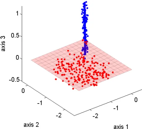
Example 3.1
For the case T = 3, n = 2, k1 = 1 and k2 = 2 we are considering a line and a
plane as two subspaces in a 3-dimensional space (See Fig.1). We have here m =
∏n
i=1(T −ki) = 2. In this case B1 is a 3×2 matrix and B2 is a 3×1 vector:
[image:10.595.174.417.319.539.2]B1 = (b11,b12) and B2 = (b21).
Figure 1: GPCA for n= 2, k1 = 1, k2 = 2, N = 200, T = 3
2
∏
i=1
||(B′ix)||=0⇐⇒p2(x) = ((b′11x)(b′21x),(b12′ x)(b′21x)) = 0. (3.11)
More concretely, for a line S1 = {x|x1 = 0, x2 = 0} and a plane S2 ={x|x3 = 0},
we have
B1 =
1 0 0 1 0 0
and B2 =
0 0 1
. (3.12)
The polynomials representing the two subspaces are:
A useful property of the polynomial representation of the subspaces is that the normal vectors of the subspaces can be obtained by differentiating the polynomials and evaluating the derivatives at one point in the respective subspaces.
For Example 3.1 the differential of p2(x) is given by:
∂p2(x)
∂x = (b11(b
′
21x) +b21(b′11x),b12(b′21x) +b21(b′12x)). (3.14)
Evaluating the differential at a pointx∈S1 with (b11,b12)′x= 0, we obtain:
∂p2(x)
∂x |x∈S1 = (b11(b
′
21x),b12(b′21x)). (3.15)
Normalizing the derivative above we obtain:
∂p2(x)
∂x |x∈S1
||∂p2(x)
∂x |x∈S1||
= (b11,b12) =B1. (3.16)
Similarly, we have
∂p2(x)
∂x |x∈S2
||∂p2(x)
∂x |x∈S2||
= (b21,b21) =B2. (3.17)
Differentiatingpn(x) to obtain the normal vectors of the subspaces provides one
way to solve for the subspaces from the data. Our question is now: how can we
obtain the polynomial pn(x), while the subspaces are still unknown? Since we have
Nsample points, each lying in one of thensubspaces, we can construct the subspaces
from the sample points. Recall that pn(x) consists of m homogeneous polynomials
of degreen in the elements ofxand each such homogeneous polynomial of degreen
is a linear combination of the monomials of the form xn11 xn22 ...xnT
T with 0≤ nj ≤ n
for j = 1, ..., T and n1+n2 +...+nT = n. Hence, we need only to find m linear
combinations of the monomials that assume the value of zero atxs that are points in
the n subspaces. To this end, we look again at Example 3.1, where the polynomial
representing the subspaces can be formulated as follows.
pn(x) = ((b′11x)(b′21x),(b′12x)(b′21x))
= ((b111x1+b112x2+b113x3)(b211x1+b212x2+b213x3),
(b121x1+b122x2+b123x3)(b211x1+b212x2+b213x3))
= (c11x21+c12x1x2+c13x1x3+c14x22+c15x2x3+c16x23,
c21x21+c22x1x2+c23x1x3+c24x22+c25x2x3+c26x23)
= (c′1ν2(x),c′2ν2(x)) = (c1,c2)′ν2(x)) = 0, (3.18)
where ν2(x) = (x21, x1x2, x1x3, x22, x2x3, x23)′ is the Veronese map of degree 2, and
the coefficients c1 is related to the normal vectors of the subspaces in the following
way: c1 = (c11, c12, c13, c14, c15, c16)′, with c11 = b111b211, c12 = b111b212 +b112b211,
c13 =b111b213+b113b211, c14=b112b212, c15=b112b213+b113b212, c16 =b113b213; and c2
is defined accordingly.
Generally, the Veronese map of degree n is defined as νn(x) : RT → RMn with
Mn=
(
n+T −1
T −1
)
. νn : (x1, ..., xT)′ →(...,xI, ...)′, wherexI =xn11 xn22 ...x nT
T with
In Example 3.1 we see that a collection of n subspaces can be described as the set of points satisfying a set of homogeneous polynomials of the form (see equation (3.18)):
p(x) =c′νn(x) = 0. (3.19)
Since each point in one of then subspaces satisfies equation (3.19), forN points in
the subspaces we will have a linear equation system:
Ln(X)c=
νn(x1)′
νn(x2)′
...
νn(xN)′
c= 0, (3.20)
whereLn(X) is an (N×Mn) matrix. Ln(X)c= 0 suggests thatccan be calculated
from the eigenvectors of the null space of Ln(X). Once we have c, we have a
representation of the subspaces as νn(x)′c = 0. This suggests further that we can
obtain the normal vectors to the subspaces by differentiating νn(x)′c with respect
to x and evaluating the derivative at points in the respective subspaces. This fact
is summarized in Theorem 5 in Vidaly (2003).
Proposition 3.2 (Polynomial differentiation Theorem 5 in Vidaly (2003)) For the GPCA problem, if the given sample setX is such that
dim(null(Ln)) = dim(In) and one generic point yi is given for each subspace Si,
then we have
Si⊥ =span
{
∂c′
nνn(x)
∂x |x=yi,∀cn ∈null(Ln) }
.
Here Si⊥ represents normal vectors of the subspace Si, Ln is the data matrix as
given in (3.20) andIn is the ideal of the algebra set pn(x) = 0 that represents the n
subspaces.
Following Proposition 3.2, the determination of the subspaces boils down to
eval-uating the derivatives of νn(x)′c at one point in each subspace. For data generated
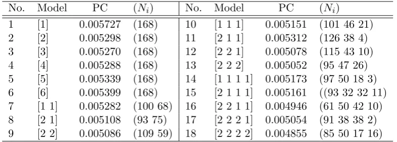
without noises, we only need to find one point in each subspace in order to calculated the normal vectors of the respective subspaces and the classification problem can be solved perfectly. This method is called polynomial differentiation algorithm(PDA) (see Vidal, Ma, and Piazzi (2004) for more details). In the following we demonstrate how PDA works in Example 3.1.
Example 3.1 (continue) We consider a set of 8 sample points from the two sub-spaces. The coordinates of the 8 points are collected in a data matrix X. Each column in X is one sample point.
X =
1 0 1 2 0 0 0 0 0 1 1 2 0 0 0 0 0 0 0 0 1 2 3 4
(3.21)
Obviously, the first four points are located in the subspace of the plane S2, and the
next four points are located in the subspace of the line S1. The Veronese mapping
Ln(X) =
1 0 0 0 0 0
0 0 0 1 0 0
1 1 0 1 0 0
4 4 0 4 0 0
0 0 0 0 0 1
0 0 0 0 0 4
0 0 0 0 0 9
0 0 0 0 0 16
. c=
0 0 0 0 1 0 0 0
0 −1
0 0
From Ln(X) we can solve for its null space by singular value decomposition. c is
the matrix containing the two eigenvectors ofN ull(Ln(X)).
The two polynomials that represent the the two subspaces can be obtained in the form of νn(x)′c=0. So we have
νn(x)′c= (x21, x1x2, x1x3, x22, x2x3, x23)c= (x1x3,−x2x3) =0.
Comparing with equation (3.13), we know νn(x)′c= 0 represents the two subspaces:
the line S1 ={x|x1 = 0, x2 = 0} and the plane S2 ={x|x3 = 0}.
According to Proposition 3.2, the normal vectors of the subspaces can be calcu-lated by evaluating
∂νn(x)′c
∂x =
∂νn(x)′c
∂x1 ∂νn(x)′c
∂x2 ∂νn(x)′c
∂x3 =
2x1 x2 x3 0 0 0
0 x1 0 2x2 x3 0
0 0 x1 0 x2 2x3
c=
x3 0
0 −x3
x1 −x2
at one point in the respective subspace. Evaluating the partial derivative at x1 tox8,
we have:
∂νn(x)′c
∂x |x1 = 0 0 0 0 1 0
, ∂νn(x)
′c
∂x |x2 =
0 0
0 0
0 −1
, (3.22)
∂νn(x)′c
∂x |x3 =
0 0
0 0
1 −1
, ∂νn(x)
′c
∂x |x4 =
0 0
0 0
2 −2
, (3.23)
∂νn(x)′c
∂x |x5 =
1 0
0 −1
0 0
, ∂νn(x)
′c
∂x |x6 =
2 0
0 −2
0 0
, (3.24)
∂νn(x)′c
∂x |x7 =
3 0
0 −3
0 0
and ∂νn(x)
′c
∂x |x8 =
4 0
0 −4
0 0
. (3.25)
Note that the rank of ∂νn(x)′c
∂x |xk corresponds to the codimension of the respective subspace and the normal vectors of the respective subspace can be calculated as the principal component of ∂νn(x)′c
∂x |xk. For the points x
1,x2,x3,x4, the principal
belong to the subspace S2 defined by the normal vector B2. The normalized
deriva-tives for points x5,x6,x7,x8 are identical. Hence these four points belong to the
subspace S1 characterized by the normal vectors B1.
B2 =
0 0 1
B1 =
1 0
0 −1
0 0
. (3.26)
3.3
Method of Generalized Principal Component Analysis
with Noisy Data
Sofar we know how to solve the classification problem if there is no noise in the data, i.e. Ei = 0 in equation (3.8). If Ei ̸= 0 several problems arise: (1) Ln(X) will have
full rank and thus equation system (3.20) has only zero solution. (2) It may happen that no point lies exactly in any one of the subspaces, such that we cannot obtain an accurate inference on the normal vectors. Yang, Rao, Wagner, Ma, and Fossum (2005) propose a PDA with a voting scheme to solve the problem with noisy data.
Algorithm 1 Generalized Principal Component Analysis
Given a set of samples {xk}Nk=1, (xk∈RK) fit an nlinear subspaces model with codimensions d1, ..., dn:
1: Set angleT olerance, letC be the number of distinct codimensions, and obtain D by the Hilbert function constraint.
2: Let V{1}, ..., V{C}be integer arrays as voting counters and U{1}, ..., U{C}
be matrix arrays for basis candidates. 3: Construct LN = [νn(x1), ..., νn(xN)].
4: Form the set of polynomials pn(x) and computeDpn(x). 5: for all samplexk do
6: for all 1≤i≤C do
7: Assume xk is from a subspace with the codimension dequal to that of the class i. Find the first dprincipal componentsB ∈RK×d in the matrixDpn(x)|
xk.
8: CompareB with all candidates inU{i}.
9: if ∃j,subspaceangle[B, U{i}(j)]< angleT olerancethen 10: V{i}(j) =V{i}(j) + 1.
11: Average the principal directions with the new basis B. 12: else
13: Add a new entry inV{i} and U{i}. 14: end if
15: end for 16: end for
17: for all 1≤i≤C do
18: m = the number of subspaces in class i.
19: Choose the first m highest votes in V{i}with their corresponding bases in U{i}. 20: Assign corresponding samples into the subspaces, and cancel their votes
in the other classes. 21: end for
The motivation of PDA with a voting scheme is the following: for a given number
of subspaces n and their codimensions {di}ni=1, the theoretical rank of the data
matrix Ln(X) called the Hilbert function constraint can be calculated. Then a set
of polynomials pn(x) with coefficients equal to the eigenvectors in the null space
of Ln(X) are formed. Through evaluating Dpn(x) at each data point, a set of
vectors normal to the subspace in which the point lies are obtained. The original PDA method relies on one good sample per subspace to classify the data. In the presence of noises, no single sample is reliable. However, through averaging the normal vectors of all samples in one subspace, it will smooth out the random noises.
The table above is the algorithm given in Yang et al. (2005)5. We demonstrate how
the PDA with a voting scheme works for Example 3.1 in the Appendix.
3.4
Classification of Variables
After obtaining a solution{Bˆ1,Bˆ2, ...Bˆn}for the subspaces, a variablexj is classified
to that subspace to whichxj has the smallest distance among all subspaces. Given
the set of estimated normal vectors {Bˆ1,Bˆ2, ...Bˆn}, we can calculate the distance
between the j-th variable xj and theith subspace ˆB
i as follows:
||ˆeji||=||Bˆ′ixj||.
The rule for classification is the following:
||eˆji||= min{||ˆej1||,||ˆej2||, ...,||ˆejn||} → xj ⇒Si, (3.27)
wherexj ⇒S
i means that xj is classified to the subspace Si.
We usexji to denote that thej-th variable is generated by the factors of thei-th
group andeji is the corresponding noise. If
||eˆjii ||= min{||eˆji1||,||ˆeji2||, ...,||ˆeji
n||} (3.28)
holds, then xji ⇒ S
i follows. This classification is correct. Assumption 2.2 implies
that if there is no noise, all data points from one group do not lie in the subspaces of other groups, so that their distances to the subspaces of other groups are always strictly positive. This ensures that the classification according to distance will lead to a unique correct classification. The existence of noises will inevitably result in some errors in the classification despite use of the voting scheme. We show how to achieve a consistent classification in the next subsection.
3.5
Projected Models
In principle, we could obtain an estimate for each subspace by PDA as described in subsection 3.3. However, the usual case of a large factor model is that the
num-ber of observations T is large and the number of overall factors k is very small.
Bi is of dimension T ×(T −ki) and the Veronese mapping matrix is of dimension
N×
(
n+T −1
T −1
)
, such that the dimension of data involved in the PDA algorithm
is very large. Consequently, the algorithm may not be practically executable due
to extremely heavy computational burdens. But, as far as classification of variables
is concerned, a large T-dimensional problem (T >> k) can be casted into a K
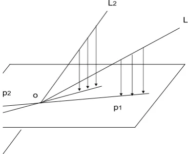
-dimensional problem with T >> K ≥ k to reduced the dimension of the problem.
The reason is that projecting the T dimensional points onto a K dimensional
sub-space that is not orthogonal to the factor sub-space, the classification is preserved6 (See
Fig.2). Hence, we can first transform theT-dimensional classification problem into
aK-dimensional classification problem with K ≥k. After solving the classification
problem, we can estimate the factors for each group using the original data.
L2
p1
L1
[image:16.595.222.415.205.363.2]p2 o
Figure 2: GPCA for n= 2, k1 = 1, k2+ 1, T = 3 andK = 2.
LetQbe the (T ×K) matrix containing the K eigenvectors corresponding toK
largest eigenvalues ofXX′. √T Q′ is a principal component estimate of factor space
spanned byG. A rescaled estimate can be calculated as follows:
ˆ
GK = 1
N T(XX
′)√T Q. (3.29)
We project the original models (2.6) and (2.4) by premultiply GˆTK to both sides of
the models and obtain:
1
TGˆ
K′
X = 1
TGˆ
K′
GΛ + 1
TGˆ
K′
E (3.30)
and
1
TGˆ
K′ Xi =
1
TGˆ
K′
FiΛi+
1
TGˆ
K′
Ei for i= 1,2, ..., n. (3.31)
Denoting T1GˆK′
X, T1GˆK′
G, T1GˆK′
E, T1GˆK′
Xi, T1GˆK
′
Fi and T1GˆK
′
Ei by ¯XT, ¯GT and
¯
ET, ¯XT
i , ¯FiT and ¯EiT respectively, we have
¯
XT
(K×N)= ¯G T
(K×k)(k×ΛN)+ ¯E T
(K×N) (3.32)
[image:16.595.83.516.575.721.2]and
¯
XiT
(K×Ni)
= F¯iT
(K×ki) Λi (ki×Ni)
+ E¯iT
(K×Ni)
for i= 1,2, ..., n (3.33)
or equivalently
¯
XiT = ˜¯XiT + ¯EiT with B¯Ti ′X˜¯iT = 0 fori= 1,2, ..., n (3.34) The projected models (3.32) and (3.33) has the following property.
Proposition 3.3
Under Assumption 2.1 to Assumption 2.7, for K =k it holds:
• (a) X¯T i
P
−→X¯i and X¯T P
−→X¯ as N → ∞, T → ∞
• (b) F¯T i
P
−→F¯i and G¯T P
−→G¯ as N → ∞, T → ∞ and F¯i = ¯GCi.
• (c) E¯T i
P
−→0 and E¯T −→P 0 as N → ∞, T → ∞
• (d) F¯i ̸= ¯Fj, for i̸=j.
• (e) F¯i is not a linear function of F¯j.
• (f ) F¯iλi,m ̸= ¯Fjλj,l for any pair of factor loadings λi,m and λj,l for m =
1,2, ...Ni, l = 1,2, ..., Nj, i= 1,2, ..., n, j = 1,2, ..., n and i̸=j.
Proof (see Appendix).
Comparing the projected model (3.33) with the original model (2.4), we see that the projected model is also a grouped factor model with the same number of groups. Proposition 3.3 (a) through (c) state that the projected model will converge to a grouped factor model without noises, i.e. all data points will eventually lie directly in the respective factor spaces. (d) through (e) state that the membership relation between variables and their groups remain preserved after projection.
Benefits of a projection from a T dimensional problem onto a K dimensional
problem are twofold: (1) it reduces the dimension of the numerical calculation in
PDA and thus makes the problem practically solvable. The dimension ofBi reduces
from{T ×(T −ki)} to{K×(K−ki)}. For a case ofT = 200, ki = 4, K = 6, and
n= 5, the number of variables in Bi reduces from 195000 to 60. (2) The projection
reduces the distance between data points and their subspaces, and thus enables a more precise classification. Eventually it will become a correct classification, as the
idiosyncratic errors converge to zero asT → ∞,N → ∞.
Since the classification rule defined in (3.27) depends on the estimated residuals, the results of the classification is stochastic. Therefore, we need to characterize the stochastic property of a classification rule.
Definition 3.4
A classification rule is called consistent if
P(||eˆjii ||= min{||ˆe1j||,||eˆj2||, ...,||ˆej
Proposition 3.5
Given a set of correct model parameters (n,{ki}ni=1), the classification rule (3.27)
based on PDA with a voting scheme applied to the projected model (3.33) withK =k
is consistent.
Proof: According to Proposition 3.3 we have ¯ET
i P
−→ 0, as T → ∞, N → ∞.
It follows ¯XT i
P
−→ X¯i, as T → ∞, N → ∞. For a variable j in ¯XiT we have
¯
xT,ji −→P x¯ji, asT → ∞, N → ∞. Let{Bˆ¯
1,Bˆ¯2, ...Bˆ¯n}be the estimate of the normal
vectors of the subspaces using PDA based on the data{X¯T
i }ni=1 and{B¯1,B¯2, ...B¯n}
be the normal vectors of the subspaces calculated with PDA based on the data {X¯i}ni=1. Because {Bˆ¯1,Bˆ¯2, ...Bˆ¯n}is a continuous function of {X¯iT}i=1n at{X¯i}ni=1, it
follows according to Slusky theorem:
{Bˆ¯1,Bˆ¯2, ...Bˆ¯n} P
−→ {B¯1,B¯2, ...B¯n},asT → ∞, N → ∞
Therefore, we have
||ˆ¯eT,jii ||=||Bˆ¯′ix¯T,ji||−→ ||P B¯′ix¯ji||= 0 as T → ∞, N → ∞,
where ˆ¯eT,jii is the distance between the data point ¯xT,ji and the estimated ith
sub-space ˆ¯Bi in the projected model (3.33) and ¯xji is the limit of ¯xT,ji asT → ∞, N →
∞. The probability limit in the equation above follows from Slusky theorem and
the last equality is due to the definition of ¯xji. Next we show that the probability
that ¯xT,ji has a strictly positive distance to other factor spaces converges to one.
1 =P(||ˆ¯eT,jil || ≥0) = P({||eˆ¯T,jil ||>0}∪{||eˆ¯lT,ji||= 0}) =P(||ˆ¯eT,jil ||>0)+P(||eˆ¯T,jil ||= 0) From Proposition 3.3 (c) and (f) we have
P(||eˆ¯T,jil ||= 0)→P(||¯ejil ||= 0) =P( ¯Flλl,j = ¯Fiλi,j) = 0, as T → ∞, N → ∞.
It follows then
P(||eˆ¯T,jil ||>0)→1 as T → ∞, N → ∞.
Because ||eˆ¯T,jii || −→P 0 and P(||eˆ¯lT,ji|| >0)−→P 1 for k ̸=i, as T → ∞, N → ∞, we have
P(¯xT,ji ⇒S¯i) = P(||eˆ¯T,jii ||= min{||eˆ¯ T,ji 1 ||,||ˆ¯e
T,ji
2 ||, ...,||ˆ¯eT,jin ||})→1, as T → ∞, N → ∞.
(3.36)
✷
Remarks: Assumption 2.2 (b) leads to the results that P(||eˆ¯jil || = 0) → 0 for
l ̸= i and hence the proof of the consistent classification above. This assumption
is, however, not essential for conducting a correct inference of the group-pervasive factors. If P(||ˆ¯ejil || = 0) > 0, a significant proportion of data would lie in the
intersection of two factor spacesiandl. Because these data lie in the intersection of
will nevertheless complicate the definition of a correct classification. In order to avoid this complication and simplify the presentation, we make Assumption 2.2 (c).
Since the membership relations between variables and their groups remain
pre-served after the projection from aT dimensional space onto aK dimensional space.
The classification of variables obtained in the projected model (3.33) is a consistent classification of the variables in the original model.
P(xji ⇒Si) = P(¯xT,ji ⇒S¯i)→1, as T → ∞, N → ∞. (3.37)
3.6
Determination of the number of groups and the number
of factors in each group
Given a set of key parameters of a grouped factor model (n,{ki}ni=1), we can classify
N variables into n groups by GPCA method. For groupi we denote theT
observa-tions of Nsn
i variables that are classified into this group by Xisn, where sn denotes
this particular grouping of the variables. If the given parameters (n,{ki}ni=1) are
cor-rect, the classification will be asymptotically correct and we can estimate, group by group, the group-pervasive factors using the standard principal component method, which is equivalent to solving of the following minimization problem:
Vi(ki,Fˆi, Nisn) = minΛ
i,Fi 1
Nsn
i T Nsn
i
∑
j=1 T
∑
t=1
(Xsn
i,jt−λi,jFi,t)2, (3.38)
where Λi = (λi,1, λi,2, ..., λi,Nsn
i ) and Fi = (Fi,1, Fi,2, ..., Fi,T)
′.
A question is now how can we know whether this set of parameters (n,{ki}ni=1)
are correct or not? One insight of Bai and Ng (2002) is that the number of factors in a group can be determined through minimizing an information criterion that consists of mean squared errors of the model and a properly scaled penalty term:
ˆ
ki = argmin0<ki≤k
(
Vi(ki,Fˆi, Nisn) + ˆσikig(Nisn, T)
)
,
whereg(Nsn
i , T) is a scaling function7.
Since we have more than one group, we need to extend the mean squared errors as well as the penalty terms over all groups. In this way we can construct a model selection criterion to determine the number of groups and the number of factors in each group. A model selection criterion,C(n,{ki}i=1n ,{Xisn}), is a scalar function of
data, model parameters and the classification of the variables, which measures the goodness of fit of the model to the data.
Definition 3.6
A model selection criterionC(n,{ki}i=1n ,{Xisn})is called consistent if it satisfies the
following condition:
P{C(no,{koi}ni=1,{Xis})< C(n′,{k′i}ni=1′ ,{Xiu})} →1 as T, N → ∞. (3.39)
Here (no {ko
i}ni=1) are parameters of the true model, and {Xis} is the corresponding
classification based on GPCA; (n′,{k′
i}n
′
i=1) are parameters of an alternative model
and {Xu
i } is the corresponding classification using GPCA.
Proposition 3.7
Under Assumption 2.1 to Assumption 2.7,
P C(n,{ki}i=1n ,{Xisn}) = n
∑
i=1
Ni
NVi(ki,Fˆ
ki, N
i)+ˆσ2
( n ∑
i=1
Ni
N (ki+h(Ni/N))
)
g(N, T)
(3.40)
is a consistent model selection criterion if the following conditions are satisfied: 1. limN→∞ NNi → αi > α, where NNi is the share of variables in the ith group. It
is to note that α is the lower bound for all candidate models.
2. g(N, T)→+0, C2
N,Tg(N, T)→ ∞ as N, T → ∞,
where CN T = min{
√
N ,√T}.
3. (a) 0< h(α)<1 for any 0≤α≤1
(b) h(αi)≥h(αj) for any 0≤αi ≤αj ≤1.
(c) ∑lαlh(αl)>
∑
jαjh(αj) for and {αj}-{αl}.
We use the notation {αj} - {αl} to present that {αj} is a finer partition of
the variables than {αl}, with ∑lαl=∑jαj = 1.
The model selection criterion can be reformulated in the following more compact form:
P C(n,{ki},{Xisn}) = ¯V({ki},{αˆi}) + ˆσ2(¯k+ ¯h)g(N, T)
where ˆσ2 is a consistent estimate of (N T)−1∑n
i=1
∑Ni
j=1
∑T
t=1E(ei,jt)2, ¯k is the
weighted average number of factors over all groups and ¯h is the weighted
aver-age of the penalty function h(ˆαi) over all groups.
Remarks
In this formulation it is clear that ¯k is the penalty due to the average number of
factors and ¯h is the penalty due to dispersion of groups. Compared to the P C
cri-terion in Bai and Ng (2002), obviously this model selection cricri-terion is a variant of
weighted average of P C criteria over all groups with an additional penalty on the
dispersion of groups in a model. Condition 1 is to make sure that the proportion of a group will not vanish asymptotically. Because we are considering the asymptotical property of the model selection criterion, the proportion of a group in a candidate model should not be vanishing. Hence we assume that for all candidate models, there exists a constant lower bound for the ratio of the number of variables in a group to the total number of variables in a model. Condition 2 is to get the right rate of convergence for the penalty term, and Condition 3 is to make sure that the average number of factors is the dominating parameter of the model and the disper-sion of groups is a dominated parameter. While comparing two models, we compare first the dominating parameters, only when the dominating parameters are equal we compare the dispersion of the groups in the two models.
A concrete choice ofg(N, T) can be:
• g(N, T) = N+TN T log(N+TN T ), and a concrete choice of h(Ni/N) is:
• h(ˆαi) = ˆ
αiN+T
ˆ
αiNT log ( ˆ
αiNT
ˆ
αiN+T )
αN+T αN T log(
αN T αN+T)
= g( ˆαiN,T)
g(αN,T),
3.7
Estimation Procedure for a Grouped Factor Model
• Step 1: Estimate k by the P C criterion of Bai and Ng (2002) using pooled
data.
• Step 2: Project the (T ×N) pooled data matrix X onto a (k×N) matrix:
¯
XT = 1
TGˆ
k′ X,
where ˆGk is defined in (3.29).
• Step 3: According to a chosen model (n,{ki}ni=1), solve for the corresponding
subspaces ( ˆ¯B1,Bˆ¯2, ...,Bˆ¯n) of the projected model (3.34) by PDA with voting
scheme and classify the variables according to rule (3.27).
• Step 4: Use the model selection criterion to evaluate alternative models to
obtain an optimal model and the corresponding classification of variables {Xsn
i }ni=1.
• Step 5: Estimate a factor model for each group of data in{Xsn
i }ni=1by the
stan-dard principal component method to obtain estimates for the respective group-pervasive factors ˆFi = Nsn1
i T(X
sn
i Xisn′)
√
T Qi, where Qi contains the ki
eigen-vectors corresponding to the ki largest eigenvalues of the matrix (XisnX sn
i
′
).
The procedure above will give a consistent classification of the variables as well as consistent estimates of the group-pervasive factor spaces.
Proposition 3.8
Under Assumption 2.1 to Assumption 2.7 and the three conditions given in Propo-sition 3.7, the procedure described above will provide a consistent estimate of the group-pervasive factor space for each group, i.e.
1
T
T
∑
t=1
||Fˆi,t−H k′
i
i Fi,t||2 P
−→0, as T → ∞, N → ∞, for i= 1,2, ...n, (3.41)
where Fˆi,t is the estimate of the group-pervasive factor of the ith group and H k′
i
i is a
(ki×ki) full rank matrix.
4
Simulation Studies and an Application
Exam-ple
4.1
Simulation Studies
In this section we document results of our simulation study. The simulation study is conducted in order to assess the performance of the proposed estimation procedure in finite sample cases. In particular we want to assess the ability of the model selection criterion in identifying the true model, i.e. the number of groups and the number of group-pervasive factors in each group. We use the number of factors
represent a GFM. For example [321|5] represents a GFM with three groups, the overall factor space is 5-dimensional and the number of factors in each group is 3, 2 and 1 respectively. To take into account that different group-pervasive factors may be correlated and hence may have common factors, our data generating process is designed in a way that there exists one common factor in all groups except the
groups with only one factor. According to this setting, in the model [321|5] there
exists one common factor in the first and the second groups and hence the overall factor space is 5-dimensional.
The data in the simulation study are generated from the following model:
Xi,jt = ki
∑
l=1
Fi,ltλi,lj+
√
θiei,jt j = 1,2, ...Ni, i= 1,2, ...n,
where the factor Fi,t = (Fi,1t, Fi,2t, ..., Fi,kit)
′ of the ith group is a (k
i ×1) vector
of N(0,1) variables; the factor loadings for the group λi,j = (λi,1j, λi,2j, ..., λi,kij)
′
is a (ki × 1) vector of N(0,1) variables; and ei,jt ∼ N(0,1). In this setting the
common component of Xi,jt has variance ki. The base case under consideration is
that the common component has the same variance as the idiosyncratic component,
i.e. θi = ki. We consider cases in which the number of groups in a GFM varies
from 2 to 4; the number of variables in each group varies from 30 to 200; and the number of observations varies from 80 to 500. These are plausible data sets for monthly and quarterly macroeconomic variables and financial variables in practical applications. In each simulation run we compare the value of the model selection criterion of the true model with those of alterative candidate models. The candidate models are chosen in a way that they include both more restrictive models and more general models in order to assess the sharpness of the model selection criterion in identifying the true model from competing model candidates. For a true model [2
2|3], [3 1] and [2 2 2] are more general models. The true model [2 2|3] consists of
two group-pervasive factor planes within a 3-dimensional overall factor space. The model [3 1] is more general because it contains a three-dimensional subspace and a one-dimensional subspace, and [2 2 2] is also more general because it contains three two-dimensional subspaces. But, [2 1] is a more restrictive model because it contains only one two-dimensional subspace and one one-dimensional subspace in a three dimensional overall factor space.
The outcomes of the simulation study are summarized in Table 1 to Table 5. The first three columns in these tables give numbers of variables in each group, total numbers of variables and numbers of observations in the respective simulation settings. The fourth column gives the true data-generating grouped factor models and the candidate models under consideration. The integers in a pair of square brackets give the numbers of factors in the respective groups of a grouped factor model. For a data-generating model we give also the dimension of the overall factor space which is the number behind the bar in the square bracket. For candidate models we do not give the dimensions of the overall factor spaces, because they will be determined in the estimation procedure. Since the estimation procedure consists
of two steps: (1) projection of the data onto ak dimensional overall factor space and
Determination of the projection dimension can be seen as a problem of compar-ing pooled ungrouped models with grouped models. The column under the header of U GRP reports the performance of the model selection criterion in this respect.
A number in the column ofU GRP gives the proportion that the correct projection
dimension is chosen and at least one grouped factor model is preferred over the cor-rectly chosen ungrouped factor model in the respective 1000 simulation runs. Since our data generating models are all grouped factor models, for a good performance of the selection criterion we expect the numbers in this column to be close to one. The
numbers in the column ofU GRP show that the model selection criterion works well
in determining the right dimension of the projection space. For all configurations
in the simulation T = 80 and Ni = 30 are enough to obtain the correct projection
dimensions, i.e. the proportions of finding the right projection dimension are very high: almost all numbers in this column are one and a few numbers below one are also close to one8.
The column under the header CCLM reports the proportion of correctly chosen
models among the candidates in 1000 simulation replications under the condition that the projection dimension is chosen correctly. Most of the numbers in the
column ofCCLM are close to one, indicating that for the considered configurations
the estimation procedure performs well in identifying the correct model from the
competing candidates, in many cases already for T ≥ 80 and Ni ≥ 30. Since the
consistence of the model selection criterion holds under T → ∞ and N → ∞, it is
not surprising that in some configurations forT = 80 and Ni = 30 the proportions
of finding the correct models are relatively low: in 5 cases the numbers are below 90% but still over 80%. However, we observe that for a given configuration the
proportion of correctly identified models approaches to one with increasing T and
Ni, forT = 150 and Ni = 60 the results are already satisfactory.
The column under the header M CLV gives the average proportion of
misclassi-fied variables in respective 1000 simulation runs. If the classification works well, the numbers in this column should be close to zero. Most of the numbers in the column ofM CLV are under 10 percent, indicating a good performance of the classification procedure. We observe that if the group-pervasive factor spaces are intersected, the share of misclassification tends to be higher. This is because as long as the group-pervasive factor spaces are intersected, data points lying close to the intersection of the group-pervasive factor spaces will lead to higher proportion of misclassification. However, because these data points are close to both group-pervasive factor spaces, this misclassification has little negative impact on estimation of group-pervasive factors.
SF F09 reports the average goodness of fit of the estimated factors to the true
factors in 1000 simulation runs. SF F0 is normalized to be between zero and one. A
number close to one implies a good fitting of the estimated factors to the true factors. Because variable classification works well, we expect also a good performance in
factor estimation. Indeed in most cases the numbers in the column of SF F0 are
over 90% and with increasingN and T, the numbers are approaching one.
8This result is consistent with the simulation result given in Bai and Ng (2002). 9SF F0 = tr(F0′Fˆ( ˆF′Fˆ)−1Fˆ′F0
)
Table 1: Estimation of grouped factor models
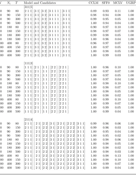
Ni N T Model and Candidates CCLM SFF0 MCLV UGRP [11|2]
30 60 80 [111] [1 1] 0.92 0.97 0.07 1.00
30 60 150 [111] [1 1] 0.97 0.97 0.05 1.00
30 60 300 [111] [1 1] 1.00 0.97 0.03 1.00
30 60 500 [111] [1 1] 1.00 0.96 0.03 1.00
60 120 80 [111] [1 1] 0.94 0.98 0.07 1.00
60 120 150 [111] [1 1] 0.97 0.98 0.05 1.00
60 120 300 [111] [1 1] 1.00 0.98 0.04 1.00
60 120 500 [111] [1 1] 1.00 0.98 0.03 1.00
200 400 80 [111] [1 1] 0.94 0.99 0.07 1.00
200 400 150 [111] [1 1] 0.99 0.99 0.05 1.00 200 400 300 [111] [1 1] 1.00 0.99 0.04 1.00 200 400 500 [111] [1 1] 1.00 0.99 0.03 1.00
[21|3]
30 60 80 [2 2 ] [2 1] [1 1] [1 1 1] [2 2 1] 0.98 0.94 0.06 1.00 30 60 150 [2 2 ] [2 1] [1 1] [1 1 1] [2 2 1] 0.99 0.95 0.04 1.00 30 60 300 [2 2 ] [2 1] [1 1] [1 1 1] [2 2 1] 1.00 0.96 0.03 1.00 30 60 500 [2 2 ] [2 1] [1 1] [1 1 1] [2 2 1] 1.00 0.95 0.03 1.00 60 120 80 [2 2 ] [2 1] [1 1] [1 1 1] [2 2 1] 0.99 0.98 0.04 1.00 60 120 150 [2 2 ] [2 1] [1 1] [1 1 1] [2 2 1] 1.00 0.98 0.03 1.00 60 120 300 [2 2 ] [2 1] [1 1] [1 1 1] [2 2 1] 1.00 0.97 0.03 1.00 60 120 500 [2 2 ] [2 1] [1 1] [1 1 1] [2 2 1] 1.00 0.98 0.02 1.00 200 400 80 [2 2 ] [2 1] [1 1] [1 1 1] [2 2 1] 1.00 0.97 0.08 1.00 200 400 150 [2 2 ] [2 1] [1 1] [1 1 1] [2 2 1] 1.00 0.97 0.09 1.00 200 400 300 [2 2 ] [2 1] [1 1] [1 1 1] [2 2 1] 1.00 0.98 0.06 1.00 200 400 500 [2 2 ] [2 1] [1 1] [1 1 1] [2 2 1] 1.00 0.99 0.04 1.00
[22|3]
30 60 80 [2 2 1] [2 1] [1 1] [1 1 1] [2 2] 0.96 0.91 0.09 1.00 30 60 150 [2 2 1] [2 1] [1 1] [1 1 1] [2 2] 1.00 0.91 0.08 1.00 30 60 300 [2 2 1] [2 1] [1 1] [1 1 1] [2 2] 1.00 0.92 0.05 1.00 30 60 500 [2 2 1] [2 1] [1 1] [1 1 1] [2 2] 1.00 0.91 0.04 1.00 60 120 80 [2 2 1] [2 1] [1 1] [1 1 1] [2 2] 0.94 0.95 0.09 1.00 60 120 150 [2 2 1] [2 1] [1 1] [1 1 1] [2 2] 0.99 0.95 0.07 1.00 60 120 300 [2 2 1] [2 1] [1 1] [1 1 1] [2 2] 1.00 0.95 0.06 1.00 60 120 500 [2 2 1] [2 1] [1 1] [1 1 1] [2 2] 1.00 0.96 0.05 1.00 200 400 80 [2 2 1] [2 1] [1 1] [1 1 1] [2 2] 1.00 0.97 0.11 1.00 200 400 150 [2 2 1] [2 1] [1 1] [1 1 1] [2 2] 1.00 0.97 0.09 1.00 200 400 300 [2 2 1] [2 1] [1 1] [1 1 1] [2 2] 1.00 0.98 0.06 1.00 200 400 500 [2 2 1] [2 1] [1 1] [1 1 1] [2 2] 1.00 0.99 0.04 1.00
Table 2: Estimation of grouped factor models
N Ni T Model and Candidates CCLM SFF0 MCLV UGRP
[32|4]
30 60 80 [3 2] [3 1] [2 1] [3 3] [3 2 1] 0.98 0.91 0.09 1.00 30 60 150 [3 2] [3 1] [2 1] [3 3] [3 2 1] 0.99 0.92 0.07 1.00 30 60 300 [3 2] [3 1] [2 1] [3 3] [3 2 1] 1.00 0.92 0.06 1.00 30 60 500 [3 2] [3 1] [2 1] [3 3] [3 2 1] 1.00 0.94 0.05 1.00 60 120 80 [3 2] [3 1] [2 1] [3 3] [3 2 1] 0.98 0.95 0.08 1.00 60 120 150 [3 2] [3 1] [2 1] [3 3] [3 2 1] 1.00 0.97 0.08 1.00 60 120 300 [3 2] [3 1] [2 1] [3 3] [3 2 1] 1.00 0.97 0.06 1.00 60 120 500 [3 2] [3 1] [2 1] [3 3] [3 2 1] 1.00 0.98 0.04 1.00 200 400 80 [3 2] [3 1] [2 1] [3 3] [3 2 1] 0.99 0.99 0.09 1.00 200 400 150 [3 2] [3 1] [2 1] [3 3] [3 2 1] 1.00 0.99 0.09 1.00 200 400 300 [3 2] [3 1] [2 1] [3 3] [3 2 1] 1.00 0.98 0.06 1.00 200 400 500 [3 2] [3 1] [2 1] [3 3] [3 2 1] 1.00 0.99 0.04 1.00
[33|5]
30 60 80 [1 1 1] [2 2] [3 2 1] [3 3 1] [3 3 2] [3 3] 0.99 0.90 0.05 0.97 30 60 150 [1 1 1] [2 2] [3 2 1] [3 3 1] [3 3 2] [3 3] 0.99 0.90 0.02 0.98 30 60 300 [1 1 1] [2 2] [3 2 1] [3 3 1] [3 3 2] [3 3] 1.00 0.90 0.01 1.00 30 60 500 [1 1 1] [2 2] [3 2 1] [3 3 1] [3 3 2] [3 3] 1.00 0.90 0.01 1.00 60 120 80 [1 1 1] [2 2] [3 2 1] [3 3 1] [3 3 2] [3 3] 1.00 0.95 0.04 1.00 60 120 150 [1 1 1] [2 2] [3 2 1] [3 3 1] [3 3 2] [3 3] 1.00 0.95 0.02 1.00 60 120 300 [1 1 1] [2 2] [3 2 1] [3 3 1] [3 3 2] [3 3] 1.00 0.95 0.01 1.00 60 120 500 [1 1 1] [2 2] [3 2 1] [3 3 1] [3 3 2] [3 3] 1.00 0.98 0.04 1.00 200 400 80 [1 1 1] [2 2] [3 2 1] [3 3 1] [3 3 2] [3 3] 1.00 0.98 0.04 1.00 200 400 150 [1 1 1] [2 2] [3 2 1] [3 3 1] [3 3 2] [3 3] 1.00 0.98 0.03 1.00 200 400 300 [1 1 1] [2 2] [3 2 1] [3 3 1] [3 3 2] [3 3] 1.00 0.98 0.02 1.00 200 400 500 [1 1 1] [2 2] [3 2 1] [3 3 1] [3 3 2] [3 3] 1.00 0.98 0.01 1.00
[31|4]
30 60 80 [2 1] [2 2] [3 2 1] [3 1 1] [3 1] 0.85 0.93 0.07 0.99 30 60 150 [2 1] [2 2] [3 2 1] [3 1 1] [3 1] 0.88 0.93 0.05 1.00 30 60 300 [2 1] [2 2] [3 2 1] [3 1 1] [3 1] 0.99 0.93 0.04 1.00 30 60 500 [2 1] [2 2] [3 2 1] [3 1 1] [3 1] 1.00 0.93 0.03 1.00 60 120 80 [2 1] [2 2] [3 2 1] [3 1 1] [3 1] 0.99 0.97 0.07 1.00 60 120 150 [2 1] [2 2] [3 2 1] [3 1 1] [3 1] 0.99 0.95 0.05 1.00 60 120 300 [2 1] [2 2] [3 2 1] [3 1 1] [3 1] 1.00 0.96 0.04 1.00 60 120 500 [2 1] [2 2] [3 2 1] [3 1 1] [3 1] 1.00 0.95 0.03 1.00 200 400 80 [2 1] [2 2] [3 2 1] [3 1 1] [3 1] 1.00 0.98 0.07 1.00 200 400 150 [2 1] [2 2] [3 2 1] [3 1 1] [3 1] 1.00 0.98 0.05 1.00 200 400 300 [2 1] [2 2] [3 2 1] [3 1 1] [3 1] 1.00 0.98 0.03 1.00 200 400 500 [2 1] [2 2] [3 2 1] [3 1 1] [3 1] 1.00 0.99 0.03 1.00
Table 3: Estimation of grouped factor models
N Ni T Model and Candidates CCLM SFF0 MCLV UGRP
[311|5]
30 90 80 [2 1 1] [3 1] [3 2] [3 1 1 1 ] [3 1 1] 0.89 0.93 0.11 1.00 30 90 150 [2 1 1] [3 1] [3 2] [3 1 1 1 ] [3 1 1] 0.98 0.94 0.08 1.00 30 90 300 [2 1 1] [3 1] [3 2] [3 1 1 1 ] [3 1 1] 0.99 0.95 0.05 1.00 30 90 500 [2 1 1] [3 1] [3 2] [3 1 1 1 ] [3 1 1] 1.00 0.94 0.04 1.00 60 180 80 [2 1 1] [3 1] [3 2] [3 1 1 1 ] [3 1 1] 0.90 0.97 0.10 1.00 60 180 150 [2 1 1] [3 1] [3 2] [3 1 1 1 ] [3 1 1] 0.98 0.97 0.07 1.00 60 180 300 [2 1 1] [3 1] [3 2] [3 1 1 1 ] [3 1 1] 0.99 0.98 0.05 1.00 60 180 500 [2 1 1] [3 1] [3 2] [3 1 1 1 ] [3 1 1] 1.00 0.96 0.04 1.00 200 400 80 [2 1 1] [3 1] [3 2] [3 1 1 1 ] [3 1 1] 0.96 0.97 0.07 1.00 200 400 150 [2 1 1] [3 1] [3 2] [3 1 1 1 ] [3 1 1] 1.00 0.97 0.05 1.00 200 400 300 [2 1 1] [3 1] [3 2] [3 1 1 1 ] [3 1 1] 1.00 0.98 0.05 1.00 200 400 500 [2 1 1] [3 1] [3 2] [3 1 1 1 ] [3 1 1] 1.00 0.99 0.03 1.00
[111|3]
30 90 80 [1 1 1] [2 1 ] [1 1 ] [2 2 ] [2 2 1 ] 1.00 0.96 0.10 1.00 30 90 150 [1 1 1] [2 1 ] [1 1 ] [2 2 ] [2 2 1 ] 1.00 0.97 0.07 1.00 30 90 300 [1 1 1] [2 1 ] [1 1 ] [2 2 ] [2 2 1 ] 1.00 0.97 0.05 1.00 30 90 500 [1 1 1] [2 1 ] [1 1 ] [2 2 ] [2 2 1 ] 1.00 0.97 0.04 1.00 60 180 80 [1 1 1] [2 1 ] [1 1 ] [2 2 ] [2 2 1 ] 1.00 0.98 0.10 1.00 60 180 150 [1 1 1] [2 1 ] [1 1 ] [2 2 ] [2 2 1 ] 1.00 0.98 0.07 1.00 60 180 300 [1 1 1] [2 1 ] [1 1 ] [2 2 ] [2 2 1 ] 1.00 0.98 0.05 1.00 60 180 500 [1 1 1] [2 1 ] [1 1 ] [2 2 ] [2 2 1 ] 1.00 0.98 0.02 1.00 200 400 80 [1 1 1] [2 1 ] [1 1 ] [2 2 ] [2 2 1 ] 1.00 0.99 0.10 1.00 200 400 150 [1 1 1] [2 1 ] [1 1 ] [2 2 ] [2 2 1 ] 1.00 0.99 0.07 1.00 200 400 300 [1 1 1] [2 1 ] [1 1 ] [2 2 ] [2 2 1 ] 1.00 0.99 0.05 1.00 200 400 500 [1 1 1] [2 1 ] [1 1 ] [2 2 ] [2 2 1 ] 1.00 0.99 0.04 1.00
[211|4]
30 90 80 [2 1 1] [ 2 1] [2 2] [3 1] [2 2 1] [2 2 2] [3 1 1] 0.99 0.96 0.06 1.00 30 90 150 [2 1 1] [ 2 1] [2 2] [3 1] [2 2 1] [2 2 2] [3 1 1] 0.99 0.96 0.03 1.00 30 90 300 [2 1 1] [ 2 1] [2 2] [3 1] [2 2 1] [2 2 2] [3 1 1] 1.00 0.95 0.04 1.00 30 90 500 [2 1 1] [ 2 1] [2 2] [3 1] [2 2 1] [2 2 2] [3 1 1] 1.00 0.95 0.02 1.00 60 180 80 [2 1 1] [ 2 1] [2 2] [3 1] [2 2 1] [2 2 2] [3 1 1] 1.00 0.98 0.06 1.00 60 180 150 [2 1 1] [ 2 1] [2 2] [3 1] [2 2 1] [2 2 2] [3 1 1] 1.00 0.98 0.05 1.00 60 180 300 [2 1 1] [ 2 1] [2 2] [3 1] [2 2 1] [2 2 2] [3 1 1] 1.00 0.98 0.02 1.00 60 180 500 [2 1 1] [ 2 1] [2 2] [3 1] [2 2 1] [2 2 2] [3 1 1] 1.00 0.98 0.03 1.00 200 400 80 [2 1 1] [ 2 1] [2 2] [3 1] [2 2 1] [2 2 2] [3 1 1] 1.00 0.98 0.13 1.00 200 400 150 [2 1 1] [ 2 1] [2 2] [3 1] [2 2 1] [2 2 2] [3 1 1] 1.00 0.98 0.10 1.00 200 400 300 [2 1 1] [ 2 1] [2 2] [3 1] [2 2 1] [2 2 2] [3 1 1] 1.00 0.99 0.07 1.00 200 400 500 [2 1 1] [ 2 1] [2 2] [3 1] [2 2 1] [2 2 2] [3 1 1] 1.00 0.99 0.04 1.00
Notes: Table 3 reports the results of 1000 Monte Carlo runs of estimation of GFMs. The first three columns give numbers of observations and numbers of variables in the respective simulation runs. The fourth columns gives the true model and the candidate models.
Table 4: Estimation of grouped factor models
N Ni T Model and Candidates CCLM SFF0 MCLV UGRP
[222|4]
30 90 80 [2 2 2] [3 2] [3 2 1] [3 2 2 ] [3 1 1] [2 1 1] 0.99 0.92 0.17 1.00 30 90 150 [2 2 2] [3 2] [3 2 1] [3 2 2 ] [3 1 1] [2 1 1] 1.00 0.93 0.13 1.00 30 90 300 [2 2 2] [3 2] [3 2 1] [3 2 2 ] [3 1 1] [2 1 1] 1.00 0.93 0.08 1.00 30 90 500 [2 2 2] [3 2] [3 2 1] [3 2 2 ] [3 1 1] [2 1 1] 1.00 0.93 0.06 1.00 60 180 80 [2 2 2] [3 2] [3 2 1] [3 2 2 ] [3 1 1] [2 1 1] 1.00 0.96 0.16 1.00 60 180 150 [2 2 2] [3 2] [3 2 1] [3 2 2 ] [3 1 1] [2 1 1] 1.00 0.97 0.11 1.00 60 180 300 [2 2 2] [3 2] [3 2 1] [3 2 2 ] [3 1 1] [2 1 1] 1.00 0.97 0.08 1.00 60 180 500 [2 2 2] [3 2] [3 2 1] [3 2 2 ] [3 1 1] [2 1 1] 1.00 0.97 0.06 1.00 200 400 80 [2 2 2] [3 2] [3 2 1] [3 2 2 ] [3 1 1] [2 1 1] 1.00 0.99 0.14 1.00 200 400 150 [2 2 2] [3 2] [3 2 1] [3 2 2 ] [3 1 1] [2 1 1] 1.00 0.99 0.11 1.00 200 400 300 [2 2 2] [3 2] [3 2 1] [3 2 2 ] [3 1 1] [2 1 1] 1.00 0.99 0.08 1.00 200 400 500 [2 2 2] [3 2] [3 2 1] [3 2 2 ] [3 1 1] [2 1 1] 1.00 0.99 0.06 1.00
[322|5]
30 90 80 [3 2 2] [4 3] [4 2] [3 3 2 ] [3 3 1 ] [3 1 1] [4 2 2] 0.92 0.91 0.16 0.97 30 90 150 [3 2 2] [4 3] [4 2] [3 3 2 ] [3 3 1 ] [3 1 1] [4 2 2] 0.96 0.92 0.11 1.00 30 90 300 [3 2 2] [4 3] [4 2] [3 3 2 ] [3 3 1 ] [3 1 1] [4 2 2] 1.00 0.92 0.07 1.00 30 90 500 [3 2 2] [4 3] [4 2] [3 3 2 ] [3 3 1 ] [3 1 1] [4 2 2] 1.00 0.93 0.06 1.00 60 180 80 [3 2 2] [4 3] [4 2] [3 3 2 ] [3 3 1 ] [3 1 1] [4 2 2] 0.99 0.98 0.13 1.00 60 180 150 [3 2 2] [4 3] [4 2] [3 3 2 ] [3 3 1 ] [3 1 1] [4 2 2] 1.00 0.96 0.11 1.00 60 180 300 [3 2 2] [4 3] [4 2] [3 3 2 ] [3 3 1 ] [3 1 1] [4 2 2] 1.00 0.96 0.07 1.00 60 180 500 [3 2 2] [4 3] [4 2] [3 3 2 ] [3 3 1 ] [3 1 1] [4 2 2] 1.00 0.96 0.05 1.00 200 400 80 [3 2 2] [4 3] [4 2] [3 3 2 ] [3 3 1 ] [3 1 1] [4 2 2] 1.00 0.99 0.12 1.00 200 400 150 [3 2 2] [4 3] [4 2] [3 3 2 ] [3 3 1 ] [3 1 1] [4 2 2] 1.00 0.99 0.09 1.00 200 400 300 [3 2 2] [4 3] [4 2] [3 3 2 ] [3 3 1 ] [3 1 1] [4 2 2] 1.00 0.99 0.08 1.00 200 400 500 [3 2 2] [4 3] [4 2] [3 3 2 ] [3 3 1 ] [3 1 1] [4 2 2] 1.00 0.99 0.05 1.00
[2222|5]
30 120 80 [2 2 2 2] [3 3] [4 2] [3 2 2 2] [2 2 2 1 ] [2 2 2 2 1 ] 0.88 0.92 0.20 0.97 30 120 150 [2 2 2 2] [3 3] [4 2] [3 2 2 2] [2 2 2 1 ] [2 2 2 2 1 ] 0.97 0.92 0.13 0.99 30 120 300 [2 2 2 2] [3 3] [4 2] [3 2 2 2] [2 2 2 1 ] [2 2 2 2 1 ] 1.00 0.93 0.11 1.00 30 120 500 [2 2 2 2] [3 3] [4 2] [3 2 2 2] [2 2 2 1 ] [2 2 2 2 1 ] 1.00 0.93 0.07 1.00 60 240 80 [2 2 2 2] [3 3] [4 2] [3 2 2 2] [2 2 2 1 ] [2 2 2 2 1 ] 0.98 0.95 0.18 1.00 60 240 150 [2 2 2 2] [3 3] [4 2] [3 2 2 2] [2 2 2 1 ] [2 2 2 2 1 ] 1.00 0.97 0.15 1.00 60 240 300 [2 2 2 2] [3 3] [4 2] [3 2 2 2] [2 2 2 1 ] [2 2 2 2 1 ] 1.00 0.96 0.10 1.00 60 240 500 [2 2 2 2] [3 3] [4 2] [3 2 2 2] [2 2 2 1 ] [2 2 2 2 1 ] 1.00 0.96 0.08 1.00 200 800 80 [2 2 2 2] [3 3] [4 2] [3 2 2 2] [2 2 2 1 ] [2 2 2 2 1 ] 1.00 0.98 0.17 1.00 200 800 150 [2 2 2 2] [3 3] [4 2] [3 2 2 2] [2 2 2 1 ] [2 2 2 2 1 ] 1.00 0.99 0.12 1.00 200 800 300 [2 2 2 2] [3 3] [4 2] [3 2 2 2] [2 2 2 1 ] [2 2 2 2 1 ] 1.00 0.99 0.09 1.00 200 800 500 [2 2 2 2] [3 3] [4 2] [3 2 2 2] [2 2 2 1 ] [2 2 2 2 1 ] 1.00 0.99 0.07 1.00