Tolls, Exchange Rates, and Borderplex International Bridge Traffic

(1)

Munich Personal RePEc Archive

Tolls, Exchange Rates, and Borderplex

International Bridge Traffic

De Leon, Marycruz and Fullerton, Thomas M., Jr. and

Kelley, Brian W.

University of Texas at El Paso

June 2009

Online at

https://mpra.ub.uni-muenchen.de/19861/

(2)

Tolls, Exchange Rates, and Borderplex International Bridge Traffic

International Journal of Transport Economics

Volume 36, 2009, Pages 223-259

Marcycruz De Leon Economic Research Department

Greater Houston Partnership Email marycruzd@hotmail.com

Thomas M. Fullerton, Jr. Department of Economics & Finance

University of Texas at El Paso El Paso, TX 79968-0543 Telephone 915-747-7747 Facsimile 915-747-6282

Email tomf@utep.edu

Brian W. Kelley

Corporate Economics Department Hunt Communities

Email brian.kelley@huntcompanies.com

Abstract

Budget constraints are forcing many governments to consider implementing tolls as a means for financing bridge and road expenditures. Newly available time series data make it possible to analyze the impacts of toll variations and international business cycle fluctuations on cross-border bridge traffic between El Paso and Ciudad Juarez. Parameter estimation is carried out using a linear transfer function ARIMA methodology. Price elasticities of demand are similar to those reported for other regional economies, but out-of-sample forecasting results are mixed.

Key Words: Bridge Traffic, Tolls, Applied Econometrics, Mexico Border

JEL Category: R41, Transportation Demand

Acknowledgements

(3)

Tolls, Exchange Rates, and Borderplex International Bridge Traffic

Introduction

During the last 100 years, most highways have been built, owned, and maintained by

governments (Geltner and Moavenzadeh, 1987). However, construction costs for new roads,

plus maintenance and enhancements to existing road networks, impose substantial public sector

budgetary pressures. Those costs can frequently exceed tax revenue capacity. As a result,

governments have been forced to look for alternative funding. One mechanism governments

have periodically considered as a means for financing the costs of construction and maintenance

of new roads is tolls (Matas and Raymond, 2003).

In the United States, tollways have been present almost since the establishment of the

nation. The first authorized private toll road in the United States, The Little River Turnpike

Company, was created in 1785 by legislation passed by the Virginia General Assembly (Newlon,

1987). Most early toll roads did not prove to be productive investments. In the 1980s, however,

tollways began to be viewed more favorably. At that time, grid deficiencies caused the public to

realize that funding constraints were affecting road maintenance efforts at all levels of

government (Federal Highway Administration, 1999).

Another reason the use of toll roads has become more widespread is that they are now

(4)

transportation demand (Ferrari, 2002). As congestion subsides, vehicle emission reductions also

occur. Furthermore, improved technology now allows electronic toll collection, which

eliminates the need for toll booths and also saves substantial amounts of time otherwise spent in

queues by motorists, at least for tolled infrastructure within countries (Federal Highway

Administration, 1999). Tolls can also be utilized to limit vehicle emissions and improve air

quality.

Because the use of tollways is becoming more prevalent, there is an expanding literature

on this general topic. Matas and Raymond (2003) state that it is of extreme importance to have

accurate knowledge of demand for toll roads for the purposes of traffic forecasting and

evaluation. That study also argues that, if the toll road industry is to grow in a cost-effective

manner, this literature must be available for government officials and private investors to utilize.

To generate accurate traffic and revenue forecasts, and to measure the effect of a toll road on a

parallel free road, then the price elasticity of demand must be known. Similar analyses are also

required for bridges.

The Borderplex economy encompasses the El Paso, USA and Ciudad Juarez, Mexico

metropolitan economies. While closely linked in an economic sense, these markets are separated

physically by the Rio Grande River, geopolitically by an international boundary, and monetarily

by separate currencies. The purpose of this paper is to examine the impacts of tolls on

cross-border regional travel patterns using newly available historical data on the international bridge

tolls charged by the City of El Paso. To achieve this, southbound commuter travel by

(5)

studied. To model these traffic categories, autoregressive-moving average (ARIMA) transfer

functions are utilized. The transfer functions model international toll bridge demand as a

function of toll prices and regional economic variables. For this analysis, monthly data from

January 1991 – December 2004 are utilized from three of the international bridges in the area.

The data include the tolls charged to pedestrians, passenger vehicles, and commercial vehicles,

along with the numbers of pedestrians, passenger vehicles, and commercial vehicles that cross

each bridge.

The next section provides an overview of previous research on toll road demand. Data

and methodology are described in the following section. Model estimation results are then

summarized. Out-of-sample forecast accuracy results are presented next. Policy implications

are then discussed. The final section includes the conclusion and suggestions for future research.

Literature Review

Because of budgetary pressures, the number of empirical analyses on tolled transportation

infrastructure has grown in recent years. Matas and Raymond (2003) study demand elasticity on

toll roads with respect to different variables that influence travel. These explanatory variables

include real gross domestic product (GDP), gasoline prices, toll price per kilometer, and a set of

dummy variables to represent changes in the road network such as improvements to parallel

roads. Parameter estimation is carried out using weighted least squares. Results indicate that toll

(6)

on the characteristics of the road itself and the alternative roads surrounding it. Not surprisingly,

demand for a toll road is more price elastic when there is an alternate free road of better quality.

In an earlier effort, Wuestefeld and Regan (1981) also conclude that each toll road is

unique and, therefore, each has a different elasticity. That study focuses on the impact of toll

increases on revenue and traffic. Multiple factors are found to affect toll road price sensitivity

such as alternate roads, trip length, trip purpose, vehicle mix, and timing of toll increases. If the

purpose of a trip is recreational, then an increase in tolls will have a greater impact on traffic than

it will have if the toll road is mostly utilized by commuters. Toll sensitivity curves are developed

to determine revenue potentials for different price increases based on previous travel patterns.

Hirschman et al. (1995) model the demand for toll bridges and tunnels in New York.

Demand is specified as a function of tolls, regional employment, motor vehicle registrations, gas

prices, and mass transit fares. Motor vehicle registrations are utilized to represent the size of the

market and mass transit fares represent an alternative to paying bridge tolls. A dummy variable

for seasonal variation is also included. Similar to other studies, parameter heterogeneity indicates

that elasticities must be estimated for each individual toll bridge since they vary even within the

same general market area. Although the elasticities vary for each bridge, all are relatively low

and the bridges that are most price sensitive are those that are near untolled roads.

Loo (2003) examines toll traffic for six tunnels in Hong Kong. A public transport

dominated city, the toll elasticities in Hong Kong are hypothesized to differ substantially from

(7)

of tolls, spatial distribution of the population, real income, gasoline prices, real parking charges,

number of private cars registered, seasonal variations, and improvements in mass transit systems.

Surprisingly, the results of the analysis indicate that toll price sensitivities in Hong Kong tunnels

(-0.103 to -0.291) are more inelastic than those of New York. Similar to empirical evidence

reported in other studies (Oum, Waters, and Yong, 1992), the low elasticity estimates indicate

that toll increases would be ineffective in reducing traffic volumes, but would raise revenue for

construction and maintenance.

Armelius (2005) analyzes congestion tolls with models that include public transport as an

alternative to toll roads and different departure times. A toll on a fast mode of transportation

(toll road) can lead to congestion on the untolled slow mode (public transportation). To avoid

congestion on public transport system, additional measures must be employed. One possibility is

to implement an integrated toll and parking policy. Cars entering the central zone during hours

when congestion is lowest would be given parking discounts. This would keep some car users

from switching to the public transport system and also reduce congestion on toll roads. Even in

cases when public transportation congestion results, tolls are still found to improve welfare. That

result is in line with earlier analyses where unpriced roads are treated as substitutes for tolled

routes (Braid, 1996; Verhoef, Nijkamp, and Rietveld, 1996).

Several studies examine the performance of congestion pricing programs that vary tolls in

order to make traffic flows more manageable (Burris, 2006; Muriello and Jiji, 2004; Olszewski

(8)

in travel times tend to be relatively small. Not surprisingly, those same characteristics also lead

to important revenue enhancements for the public agencies managing the roads and bridges in

question. Many of the results documented confirm conclusions pointed to by separate research

involving optimal pricing strategies (Miniason, 1979; Yang and Bell, 1996; Yildirim and Hearn;

2002).

Other studies examine factors that influence the political acceptability of toll roads and

bridges (Lave, 1994; Brownstone et al., 2003; Raux and Souche, 2004). Among the various

items that affect whether residents will support tolls are geographic market size and willingness

to charge higher tolls for cargo vehicles. Capacity constraints on existing parallel roads

increases the likelihood of toll infrastructure approvals. In many regions, it is ultimately funding

constraints that convince stakeholders to turn to tolled facilities as a means for addressing

network congestion and bottlenecks (Podgorski and Kockelman, 2006).

There have been several analyses of international bridge traffic in the El Paso and Ciudad

Juarez Borderplex regional economy (Villegas et al., 2006). Fullerton (2001) builds a structural

econometric model of the Borderplex economy that examines the impacts of population,

incomes, and maquiladora manufacturing growth on annual bridge volumes. In turn, those

traffic flows affect various categories of retail sales activity on the north side of the river.

Fullerton (2004) tabulates the historical accuracies of the various annual frequency bridge traffic

category econometric forecasts published every year by the University of Texas at El Paso.

(9)

border crossings. Fullerton and Tinajero (2002) also use monthly frequency data to analyze

northbound cargo flows.

None of the studies to date on this topic examine the impact of tolls on cross-border

bridge traffic. Toll collections, however, represent an important source of municipal revenue in

El Paso (www.ci.el-paso.tx.us, accessed 19 March 2007). This study attempts to partially fill

that gap by analyzing southbound traffic volumes across tolled international bridges connecting

El Paso, Texas and Ciudad Juarez, Chihuahua. Completion of the analysis is now feasible due to

newly available historical time series data regarding southbound bridge flows and the tolls

charged to each respective traffic category. In addition to bridge tolls, the analysis also examines

the roles played by inflation adjusted (real) exchange rate movements and business cycle

fluctuations.

Data and Methodology

In December 2004, more than 19.7 thousand pedestrians, 13.3 thousand cars, and 710

cargo trucks used the tolled international bridges linking El Paso and Ciudad Juarez on a daily

basis. During fiscal year 2006, the fees for using that infrastructure generated more than $14.2

million for the El Paso city budget (www.ci.el-paso.tx.us, accessed 19 March 2007). To date,

however, an empirical analysis of the various traffic categories that pay those tolls charged on

international bridge use in El Paso has not previously been attempted. Time series data for

(10)

data for the corresponding northbound traffic out of Mexico have not yet been compiled and are,

thus, excluded from the analysis.

Different types of users are associated with the various bridges. For example, the Santa

Fe Bridge near downtown El Paso is typically used by pedestrian tourists from the United States

who want to visit Mexico without driving. The nearby Stanton Bridge is traversed primarily by

students, shoppers, and workers who reside in Ciudad Juarez and commute between the two

border cities either by car or on foot. The Zaragoza International Bridge mostly carries two types

of southbound traffic. One is cargo vehicles headed to maquiladora plants in the eastern

quadrants of Ciudad Juarez or farther south in the state capital of Chihuahua City. The second is

working professionals who commute to jobs on the opposite side of the border from where they

reside.

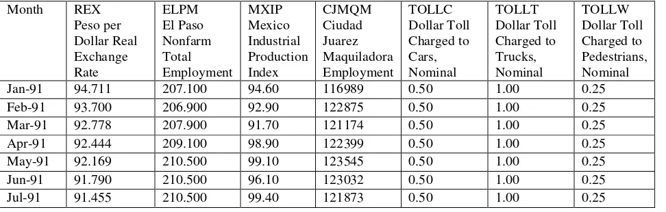
Data utilized for this analysis are from three of the international bridges in the

Borderplex: Santa Fe, Stanton, and Zaragoza. Monthly data gathered from the international

bridges include the numbers of pedestrians, passenger vehicles, and commercial vehicles, plus

the respective tolls paid by each group. The sample period is January 1991 to December 2004.

The information is collected by the City of El Paso Streets Department and reported by the City

of El Paso Office of Management and Budget. Those time series, plus others employed in the

study, are shown in Appendix Tables A1 and A2 below. As shown in the data tables, the tolls

charged for each traffic category generally remain fixed in nominal terms for long periods of

(11)

Other data utilized include Ciudad Juarez maquiladora employment, Mexico Industrial

Production Index, El Paso non-agricultural employment, United States consumer price index

(CPI), and a real exchange rate index for the peso. The CPI and El Paso monthly employment

data are reported by the United States Bureau of Labor Statistics (www.bls.gov, accessed 19

October 2006). The Mexico industrial production index and Ciudad Juarez in-bond

manufacturing employment data series are available from the INEGI national statistics website

(www.inegi.gob.mx, accessed 14 November 2006). The inflation adjusted peso index is from the

University of Texas at El Paso Border Region Modeling Project (Fullerton and Tinajero, 2002).

The 14-year sample period spans a long enough period to contain expansion, recession,

and recovery phases of the national business cycles in both the United States and Mexico. With

a total of 168 observations, the sample is sufficiently large to permit time series analysis of the

data in question (Wei, 1990). Because El Paso and Ciudad Juarez are both growing fairly

rapidly, the data used in this and other studies of cross-border bridge transportation are

non-stationary (Fullerton, 2000). Given that, the variables are differenced prior to modeling (Pindyck

and Rubinfeld 1998).

Empirical analyses for each series are completed using linear transfer function (LTF)

ARIMA procedures. Cross correlation functions are used to identify the potential lag structures

for each equation. Once parameter estimation has been completed for a particular lag structure,

diagnostic statistics are utilized to examine its performance. Among the latter, an autocorrelation

(12)

fail to capture. An LTF for a dependent variable y with multiple lags of two explanatory

variables, x and z, plus autoregressive and moving components, can be expressed as follows:

1. yt = θ0 +

=

p

i 1

φiyt-i +

=

q

j 1

θjet-j +

=

n

a 1

Aaxt-a +

=

k

b 1

Bbzt-b + et .

LTF procedures frequently perform well when used to analyze model time series data.

Because it emphasizes the relationships between the dependent variable of interest and potential

explanatory variables, it has been used in numerous econometric settings. Several examples are

from regulated markets such as residential natural gas consumption, electricity consumption, and

municipal water consumption dynamics. In addition to good in-sample estimation diagnostics,

many studies also indicate that LTF models often exhibit reliable out-of-sample simulation

properties. In at least one instance, an LTF modeling approach has been utilized to analyze

cross-border bridge traffic, albeit without taking into account the effects of toll changes

(Fullerton and Tinajero, 2002).

Individual LTF equations are estimated for each bridge and traffic category. The five

equations include cars heading south across the Zaragoza Bridge (ZC), cargo trucks using the

Zaragoza Bridge (ZT), pedestrians utilizing the Stanton Bridge (STW), cars using the Stanton

Bridge (STC), and pedestrians crossing the Santa Fe Bridge (SFW) into Mexico. In the

equations, demand for the use of the toll bridges is modeled as a function of lags of the relevant

(13)

production in Mexico (MXIP), the real exchange rate (REX), and El Paso employment (ELPM).

Implicit functions for each traffic category can be expressed as follows:

2. Traffict = f (TOLLt-i, CJMQMt-j, MXIPt-k, REXt-m, ELPMt-n, ARt-p, MAt-q).

(-) (+) (+) (?) (+)

The arithmetic signs in the parentheses below Equation 2 represent the overall

hypothesized relationship between the left-hand side variable and each independent variable.

The deflated toll series obviously serve as real price variables for each respective equation and

will tend to reduce bridge usage when they increase (Hirschman et al., 1995). The sign

underneath the inflation adjusted peso index is ambiguous. While depreciation of the peso

generally leads to reduced numbers of Mexican pedestrians and automobiles, it also generates

increased volumes of cross-border cargo traffic and tourists from the United States (Fullerton,

2000).

Monthly income data are not available for either Borderplex city. Given that, alternative

business cycle indicators are employed. For El Paso, total non-agricultural employment provides

a fairly inclusive measure of economic conditions on the north side of the river. Because no

similar broad metric is available for Ciudad Juarez, two variables are utilized. They are in-bond

manufacturing payroll employment and the Mexico industrial production index (Fullerton and

Tinajero, 2002). Transfer ARIMA models assume unidirectional causality from the explanatory

(14)

employed below violate this assumption. Empirical estimation results from the various models

are discussed in the next section.

Estimation Results

Tables 1 through 5 summarize the estimation results for each of the different bridge

traffic categories. Due to trend non-stationarity, all of the series are differenced prior to

estimation. Following parameter estimation, the series are brought back to level form and a

pseudo R-squared is calculated for each equation. A price elasticity of demand is also calculated

for each model.

Table 1 summarizes the results from the linear transfer function estimated for cargo

vehicles utilizing the Zaragoza Bridge. An increase in the toll leads to a decrease in cargo traffic

within one month of implementation. Ciudad Juarez maquiladora employment, the Mexico

industrial production index, and the real exchange rate are all positively correlated with cargo

vehicle traffic on the Zaragoza Bridge. A devaluation of the peso leads to a rapid increase in

cargo vehicle traffic. Four of the eight parameters in this equation fail to satisfy the 5-percent

significance criterion, but the F-statistic is significant at the 1-percent level. That may reflect the

presence of multicollinearity such as what has been noted in other border econometric studies

(Fullerton and Tinajero, 2002). With the lone exception of the real exchange rate index, the

(15)

the other four explanatory variable range between 0.79 and 0.93. The pseudo coefficient of

determination is 0.812. As shown in Table 6, the price elasticity calculated for this model is

-0.474 implying that cargo vehicle traffic is not very responsive to changes in the toll. Because

there are only two international bridges that carry trucks directly into Ciudad Juarez, the

inelasticity with respect to the toll is not surprising (Graham and Glaister, 2004).

The results for Zaragoza Bridge passenger vehicles are given in Table 2. In this equation,

Zaragoza Bridge passenger vehicle traffic is positively correlated with El Paso employment,

Ciudad Juarez maquiladora employment, and the Mexico industrial production index. The

inflation adjusted toll and real exchange rate are negatively correlated with passenger vehicle

traffic. That a devaluation of the peso leads to a decrease in passenger vehicle traffic probably

reflects the loss of purchasing power experienced by Mexican shoppers who visit large shopping

centers such as Cielo Vista Mall and Las Palmas Marketplace in East El Paso. The pseudo

R-squared for this equation is also relatively high, 0.813. The price elasticity of demand reported

in Table 6 for Zaragoza Bridge passenger vehicles is -0.0035. That indicates that passenger

vehicle traffic on this bridge reacts very little to increases in the toll paid by cars. While the

failure of the toll coefficient to satisfy the 5-percent significance criterion means that result

should potentially be treated with caution, similarly low elasticities have also been documented

for other regions (Wuestefeld and Regan, 1981; Hirschman et al., 1995; Loo, 2003).

Multicollinearity may also affect these results. With the exception of the real exchange rate

index, the simple correlation coefficients between the real toll for cars and the four remaining

(16)

Stanton Bridge passenger vehicle results are reported in Table 3. In this model,

passenger vehicle traffic flows are inversely related to the real toll and exchange rate variables.

The sign of the real peso parameter potentially reflects the proximity of this bridge to the

downtown retail sector on the north side of the border (Villegas et al., 2006). El Paso

employment, Ciudad Juarez in-bond assembly employment, and the Mexico industrial

production index are positively correlated with volume of cars that travel across the artery. With

a pseudo coefficient of determination of 0.889, the model explains a relatively high percentage of

the variation in passenger vehicle traffic on the Stanton Bridge. As with the other traffic

categories, the price elasticity of demand of -0.278 indicates that the number of vehicles heading

south on this artery is not strongly affected by increases in the toll. It is also similar to what has

been documented for other markets (Matas and Raymond, 2003).

Results for the Stanton Bridge pedestrian equation are summarized in Table 4. Large

numbers of shoppers who cross on foot from Mexico return home over this structure. Not

surprisingly, southbound pedestrian traffic flows on this bridge are inversely related to changes

in the inflation adjusted values of the toll and the exchange rate. El Paso non-agricultural jobs,

Ciudad Juarez maquiladora employment, and the Mexico industrial production index are all

positively correlated with pedestrian traffic on the Stanton Bridge. The pseudo R-squared for

(17)

variation in the dependent variable for the sample period in question. Most pedestrian travel

studies do not examine the impacts of tolls on this traffic category (Hoogendoorn and Bovy,

2005). While a comparison to other estimates is not, therefore, possible, the -0.482 price

elasticity measured for this bridge seems fairly reasonable. As with the truck and automobile

equations, multicollinearity may affect the pedestrian modeling results. With the exception of

the real exchange rate index, the simple correlation coefficients between the inflation adjusted

pedestrian toll and the other independent variables ranges between 0.72 and 0.91.

The results for Santa Fe Bridge pedestrians are given in Table 5. Pedestrian traffic is

inversely related to changes in real toll along this bridge. For all other explanatory variables, the

regression coefficients carry positive signs. For the real exchange rate, that means that peso

depreciation leads to an increase in foot traffic to the downtown Ciudad Juarez tourist district.

This bridge is the one that most visitors from the United States use when they walk across the

border. The response is more rapid than what is separately reported for total commuter flows

(Fullerton, 2000). A stronger dollar probably attracts tourists who visit entertainment venues,

restaurants, and shops, as well as medical tourists who are customers at the many health facilities

and pharmacies located in this sector of the city. The pseudo coefficient of determination is

0.73. A price elasticity of -0.483 is estimated for Santa Fe Bridge pedestrians, almost identical to

that calculated for pedestrians that utilize the Stanton Bridge, even though the two series respond

(18)

The passenger and cargo vehicle price elasticities shown in Table 6 are similar in

magnitude to many of those reported over time in the transport economics literature (Wuestefeld

and Regan, 1981; Hirschman et al., 1995; Matas and Raymond, 2003). One area in which some

uncertainty remains for Table 6 is that comparative results for pedestrian reactions to changes in

tolls have not been documented elsewhere. Another source of uncertainty regarding the

information in Tables 1 through 6, and not already discussed above, is the absence of variables

that reflect the availability of alternative routes that are not subject to tolls (Braid, 1996). Due to

the distances involved, realistic untolled international bridge choices only exist for passenger and

cargo vehicles. Experimentation with a combination of traffic volume and population estimates

did not yield coefficients in any of the equations that satisfied the 5-percent significance

criterion. The various traffic volume measures included totals for all bridges, as well as for the

untolled Bridge of the Americas alone.

Results in Tables 1 through 6 are comparable to those reported elsewhere and seem fairly

reasonable from an economic perspective (McCloskey and Ziliak, 1996). However, good

in-sample traits do not always guarantee reliable out-of-in-sample simulation performance (Leamer,

1983). For municipal revenue models, forecast performance is an important question that

(19)

such an exercise has ever been completed for bridge tolls collected at international borders.

Results of such an effort using the LTF traffic models are discussed below.

Comparative Simulation Results

Following LTF parameter estimation, forecasts are generated in rolling 12-month

increments over the period covering January 2001 to December 2004 for each bridge category.

Predictive accuracy for these forecasts is assessed relative to random walk benchmarks. The

random walk (RW) forecasts are assembled using the last actual sample observations for each

traffic category. To evaluate the performances of the two forecast categories, three different

metrics are employed: a descriptive U-statistic (Pindyck and Rubinfeld, 1998), a non-parametric

t-test (Diebold and Mariano, 1995), and a regression based F-test (Ashley, Granger,

Schmalensee, 1980).

Out-of-sample simulations for the linear transfer function and corresponding random

walks are generated in the same manner. For the first set of predictions, a historical sample

period is defined from January 1990 to December 2000. The first simulation conducted is from

January 2001 to December 2002. The historical sample period is then extended by one month to

include January 2001 and the new forecast period is February 2001 to January 2003. This rolling

forecast procedure is conducted sequentially through December 2004. This yields a total of 48

(20)

The first measure utilized to compare the LTF and RW forecasts is the U-statistic or

Theil inequality coefficient. A U-statistic scales the root mean square error for a forecast such

that it ranges between 0 and 1 (Pindyck and Rubinefeld 1998). The second accuracy measure is

based on an error differential regression test (AGS) conducted at different step lengths (Ashley,

Granger, and Schmalensee 1980). The third accuracy metric employs a non-parametric t-test

(DM) based on the differences between RW and LTF root mean square errors (Diebold and

Mariano, 1995).

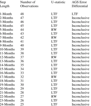
Results for the Zaragoza cargo vehicles forecasts are summarized in Table 7. The

descriptive U-statistics favor the LTF out-of-sample simulations in 19 of the 24 individual

step-lengths for this traffic category. The DM procedure also indicates that the LTF root mean square

errors (RMSEs) are significantly lower than the RW RMSEs across all step-lengths. The AGS

test outcomes for southbound truck travel on this bridge are much less decisive. Only in the case

of the single month-ahead forecasts did the AGS test point to LTF predictive superiority. For all

other 23 step-lengths, the AGS results are statistically inconclusive. Accordingly, some caution

appears warranted with respect to using the LTF equation in operations planning or revenue

forecasting applications for cargo vehicle usage of the Zaragoza Bridge.

Table 8 reports the forecast rankings for Zaragoza Bridge passenger vehicles. Results for

the descriptive inequality coefficient point to LTF relative forecast accuracy across all

(21)

AGS regression tests. Not surprisingly, the DM t-test also yields evidence that the LTF RMSEs

are significantly smaller than those of the RW passenger flow to Mexico forecasts via this

bridge. These outcomes offer partial confirmation that the price elasticity reported for this

bridge usage category in Table 6, while still relatively low, may be accurate.

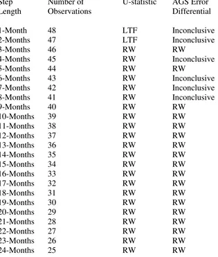
The Stanton Bridge near the downtown region of El Paso also carries passenger vehicle

traffic. As shown in Table 9, the out-of-sample simulation results for this variable are very

different from those for passenger vehicles in East El Paso. The LTF equation obtains lower

U-statistics for the one-month and two-month ahead forecasts. For the AGS error difference

regression tests, the evidence against the LTF simulations is also very pronounced. In six cases,

the results are inconclusive. For the other 18 step-lengths, significantly better prediction

accuracy is recorded for the RW forecasts. The DM t-test also points to lower RMSEs for the

RW passenger vehicle benchmarks for this commuter category.

The Stanton Bridge also provides southbound pedestrians entry into Mexico. Table 10

lists the relative predictive accuracies of the LTF equation and the RW procedure. The

inequality coefficients are lower at every step-length for the RW forecasts. For the AGS

(22)

clear cut as the AGS column of Table 10 indicates. That is because the DM t-test for RMSE

equality across all 24 step-lengths is inconclusive.

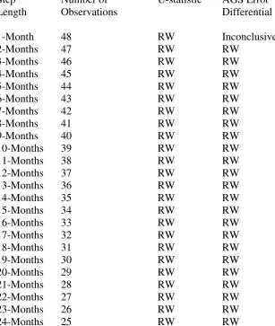
Pedestrians can also cross the Santa Fe Bridge into Mexico. The out-of-sample

simulation rankings in Table 11 document the academic equivalent of a forecast shutout on

behalf of the RW extrapolations. Both the descriptive U-statistics and the AGS test outcomes

indicate relative LTF inaccuracy at all 24 step-lengths. The DM t-test also documents

statistically smaller RMSEs across all step-lengths.

The out-of-sample simulation results imply that the LTF model achieves greater accuracy

than the RW benchmarks for both the Zaragoza Bridge cargo vehicle and the Zaragoza Bridge

passenger vehicle forecasts. However, the comparative test statistics also indicate that the RW

predictions are more accurate than the LTF forecasts for southbound pedestrian traffic flows

across the Stanton Bridge and the Santa Fe Bridge. It is somewhat more difficult to interpret the

accuracy ranking for the passenger vehicle flows across the Stanton Bridge, but the overall

evidence favors the RW benchmark at the expense of the LTF model. These mixed results are

similar to those previously reported by Fullerton (2004) using annual frequency data and call for

some care to be used with regard to employing the LTF estimates in public administrative

(23)

Policy Implications

Several results from the analysis above can potentially be of use to policy makers. Given

that all five categories of bridge traffic are inelastic with respect to the respective tolls charged,

rate increases will raise revenues without substantial reductions in volume usage. Although it

would be politically, and diplomatically, difficult to use international bridges connecting the

United States and Mexico as “cash cows,” the City of El Paso should be capable of covering a

substantial portion of current maintenance and future structural enhancement costs with the tolls

charged. At one point, there was a 9-year period from November 1994 to December 2003 during

which passenger vehicle tolls were left unchanged in nominal terms. There is no need to allow

real erosion of the tolls to occur for such a long time. All three user fees can be adjusted more

frequently without damaging the respective revenue streams. Given the rapid growth of

international commerce in this region, plus the strong rates of population and economic

expansion in the Borderplex, raising tolls provides one means for financing the infrastructure

expansion and upgrades that will undoubtedly become necessary in future years.

The lag structures in each equation are also of interest from a public administration

standpoint. All of the traffic categories respond within 60 days or less to toll rate changes.

Cargo traffic across the Zaragoza bridges reacts in less than 30 days to variations in in-bond

assembly payrolls and industrial production activity in Mexico. Staffing levels at that bridge will

(24)

currency value of the peso and non-agricultural employment in El Paso. Accordingly, flexible

staffing schedules will have to be maintained in order to maximize efficiencies and revenues at

these international exit points from El Paso. Because the price reactions are inelastic, raising

tolls at the bridges would probably not be very effective as a means for reducing vehicle

emissions via reduced traffic flows.

Given the mixed outcomes for the comparative out-of-sample simulation results, the LTF

models should be used with caution in municipal revenue forecasting endeavors. This is

especially true for the two downtown international bridges that charges tolls on southbound

traffic to Ciudad Juarez. At a minimum, LTF traffic forecasts should be compared to recent

historical observations as a means of providing “sanity checks” for the extrapolation results.

During periods in which rate increases are enacted, policy analysts may elect to rely more

heavily on the LTF model simulations since those equations provide a quantitatively systematic

manner for anticipating potential bridge usage impacts.

To date, the City of El Paso has only used fixed toll schedules. That is probably because

nearly all of the congestion that occurs on the international bridges is experienced by northbound

traffic heading into El Paso. The latter circumstance is largely due to more time consuming

inspection practices historically applied by the United States at its ports of entry. It is possible,

however, that Borderplex economic and demographic expansion may also lead to capacity

constraints on the southbound lanes of the tolled bridges. Should that eventuality come to pass,

variable congestion tolls might offer a viable mechanism for managing the greater traffic flow

(25)

schedules now in place, however, may be good choices for a regional road network already split

in two by an international boundary (Bonsall et al., 2007).

Tolls remain a highly controversial topic in El Paso and other parts of Texas (Podgorski,

and Kockelman, 2006; Crowder, 2007). State government funding constraints increase the

likelihood that a portion of the road network in El Paso may one day be funded with tolls.

Econometric analysis of the long history of charging tolls on three of the international bridges

indicates that local traffic behavior patterns are similar to those documented for other regional

economies where these user fees are charged. Based on that, it would appear that employing

tolls to partially fund the street and highway grid in El Paso should meet with success.

Conclusion

As road construction and maintenance costs continue to increase, governments

periodically look to tolls as a means of financing roadway construction and improvements.

Although tolls have been charged on three of the international bridges linking El Paso and

Ciudad Juarez for many years, empirical assessment of the impacts of those fees on traffic

patterns had not previously been completed. This study takes advantage of newly available

monthly historical toll data for El Paso to examine this aspect of the Borderplex economy.

A linear transfer function methodology is used to model toll bridge demand as a function

(26)

exchange rate. Individual equations are estimated for each of the five traffic categories that pay

the bridge user fees. As with other transfer function studies, multicollinearity appears to be

present, but overall in-sample diagnostics are relatively favorable. The price elasticities of

demand are similar in magnitude to those calculated for other regional economies. Mixed

results, however, are obtained for the out-of-sample model simulation exercises. Given that,

caution should be used if the equations are applied in municipal revenue forecasting tasks.

Data constraints currently prevent analyzing the impacts of tolls on northbound

international bridge traffic into El Paso, but eventual comparative analyses for the other side of

the river would be helpful. It would also be interesting to examine whether the results for

southbound traffic out of El Paso into Mexico can be replicated using data for other border

metropolitan economies. Potential examples include San Diego – Tijuana, Calexico – Mexicali,

Douglas – Agua Prieta, Laredo – Nuevo Laredo, McAllen – Reynosa, and Brownsville –

Matamoros. Additional toll bridge research for other regions would also be useful due to the

relatively small amount of research currently available for this topic.

References

Armelius, H. “An Integrated Approach to Urban Road Pricing.” Journal of Transport Economics & Policy, 39, 2005, 75-92.

Ashley, R., C.W.J. Granger, and R. Schmalensee. “Advertising and Aggregate Consumption: An Analysis of Causality.” Econometrica, 48, 1980, 1149-1167.

(27)

Braid, R.M. “Peak-Load Pricing of a Transportation Route with an Unpriced Substitute.” Journal of Urban Economics 40, 1996, 179-197.

Brownstone, D., A. Ghosh, T.F. Golob, C. Kazimi, and D. Van Amelsfort. “Drivers’ Willingness-to-Pay to Reduce Travel Time: Evidence from the San Diego I-15 Congestion Pricing Project.” Transportation Research A, 37, 2003, 373-387.

Burris, M.W. “Incorporating Variable Toll Rates in Transportation Planning Models.”

International Journal of Transport Economics 33, 2006, 351-368.

Chang, S. “Municipal Revenue Forecasting.” Growth and Change, 10, 1979, 38-46.

Crowder, D. “Mobility Authority Established.” El Paso Times, 14 March 2007, B1.

Diebold, F.X., and R.S. Mariano. “Comparing Predictive Accuracy.” Journal of Business and Economic Statistics, 13, 1995, 253-263.

Federal Highway Administration. “Toll Facilities in the United States.” Publication FHWA-PL-99-011. Washington, DC: U.S. Department of Transportation, 1999.

Ferrari, P. “Road Network Toll Pricing and Social Welfare.” Transportation Research B, 36, 2002, 471-483.

Forrester, J.P., “Budgetary Constraints and Municipal Revenue Forecasting.” Policy Sciences, 24, 1991, 333-356.

Fullerton, T.M., Jr. “Currency Movements and International Border Crossings.” International Journal of Public Administration, 23, 2000, 1113-1123.

Fullerton, T.M., Jr. “Specification of a Borderplex Econometric Forecasting Model.” International Regional Science Review, 24, 2001, 245-260.

Fullerton, T.M., Jr. “Borderplex Bridge and Air Econometric Forecast Accuracy.” Journal of Transportation & Statistics, 7, 2004, 7-21.

Fullerton, T.M., Jr., and R. Tinajero. “Cross Border Business Cargo Vehicle Flows.”

International Journal of Transport Economics, 29, 2002, 201-2132.

Geltner, D., and F. Moavenzadeh. “An Economic Argument for Privatization of Highway Ownership.” Transportation Research Record,1107, 1987, 14-20.

Graham, D.J., and S. Glaister. “Road Traffic Demand Elasticity Estimates: A Review.”

(28)

Hirschman, I., C. McKnight, J. Pucher, R.E. Paaswell, and J. Berechman. “Bridge and Tunnel Toll Elasticities in New York.” Transportation, 22, 1995, 97-113.

Hoogendoorn, S.P., and P.H.L. Bovy, “Pedestrian Travel Behavior Modeling.” Networks & Spatial Economics, 5, 2005, 193-216.

Lave, C. “The Demand Curve under Road Pricing and the Problem of Political Feasibility.”

Transportation Research A, 28, 1994, 83-91.

Leamer, E.E. “Let’s take the Con out of Econometrics.” American Economic Review, 1983, 73, 31-43.

Loo, B.P.Y. “Tunnel Traffic and Toll Elasticities in Hong Kong: Some Recent Evidence for International Comparisons.” Environment & Planning A, 35, 2003, 249-276.

Matas, A., and J.L. Raymond. “Demand Elasticity on Tolled Motorways.” Journal of Transportation & Statistics, 6, 2003, 91-108.

McCloskey, D.N., and S.T. Ziliak. “The Standard Error of Regressions.” Journal of Economic Literature, 1996, 34, 97-114.

Minasian, J. “Indivisibility, Decreasing Cost, and Excess Capacity: The Bridge.” Journal of Law & Economics, 22, 1979, 385-397.

Muriello, M.F., and D. Jiji. “Value Pricing Toll Program at Port Authority of New York and New Jersey – Revenue Management for Transportation Investment and Incentives for Traffic Management,” Transportation Research Record 1864, 2004, 9-15.

Newlon, H. “Private Sector Involvement in Virginia’s Nineteenth-Century Transportation Improvement Program” Transportation Research Record 1107, 1987, 3-13.

Olszewski, P., and L.T. Xie. “Modelling the Effects of Road Pricing on Traffic in Singapore.”

Transportation Research A, 39, 2005, 755-772.

Oum, T.H., W.G. Waters, and J.S. Yong. “Concepts of Price Elasticities of Transport Demand and Recent Empirical Estimates – An Interpretative Survey.” Journal of Transport Economics & Policy, 26, 1992, 139-154.

Pindyck, R.S., and D.L. Rubinfeld, D. Econometric Models and Economic Forecasts. 4th Edition. New York, NY: Irwin McGraw-Hill, 1998.

(29)

Raux, C., and S. Souche. “The Acceptability of Urban Road Pricing.” Journal of Transport Economics & Policy, 38, 2004, 191-215.

Verhoef, E., P. Nijkamp, and P. Rietveld, “Second-Best Congestion Pricing: The Case of an Untolled Alternative.” Journal of Urban Economics, 40, 1996, 279-302.

Villegas, H., P.L. Gurian, J.M. Heyman, A. Mata, R. Falcone, E. Ostapowicz, S. Wilrigs, M. Petragnani, and E. Eisele. “Trade-offs between Security and Inspection Capacity – Policy Options for Land Border Ports of Entry.” Transportation Research Record 1942, 2006, 16-22.

Wei, W. Time Series Analysis: Univariate and Multivariate Methods. Redwood City, CA: Addison-Wesley, 1990.

Wuestefeld, N.H., and E.J. Regan. “Impact of Rate Increases on Toll Facilities.” Traffic Quarterly, 35, 1981, 639-655.

Yang, H., and M.G.H. Bell. “Traffic Restraint, Road Pricing, and Network Equilibrium.”

Transportation Research B, 31, 1997, 303-314.

(30)

[image:30.612.67.500.94.324.2]

TABLE 1, Zaragoza Bridge Cargo Vehicles, ZT

Variable Coefficient Std. Error t-Statistic Probability Constant -0.136059 0.222145 -0.612477 0.5412 TOLLT(-1) -81.30670 586.0849 -0.138729 0.8899 CJMQM 0.000172 6.32E-05 2.714161 0.0075 MXIP 0.201084 0.045524 4.417113 0.0000 MXIP(-5) 0.084077 0.035686 2.355987 0.0198 MXIP(-12) 0.133327 0.041862 3.184887 0.0018 REX 0.018559 0.039964 0.464402 0.6431 AR(2) 0.111979 0.079043 1.416676 0.1587

R-Squared 0.448186 Dependent Variable Mean 0.042170 Pseudo R-Squared 0.812798 Dependent Variable Std. Deviation 3.166322 Std. Err. Regression 2.408182 Akaike Information Criterion 4.646492 Sum Sq. Residuals 840.9041 Schwarz Information Criterion 4.804946 Log-Likelihood -347.4566 F-Statistic 16.82424 Durbin Watson Stat. 2.747830 F-Statistic Probability 0.000000

Linear Transfer Function Table Notes:

Sample Period, January 1991 – December 2004. ZT, Zaragoza Bridge monthly cargo truck traffic. ZC, Zaragoza Bridge monthly passenger car traffic. STC, Stanton Bridge monthly passenger car traffic. STW, Stanton Bridge monthly pedestrian traffic. SFW, Santa Fe Bridge monthly pedestrian traffic.

TOLLT, inflation adjusted cargo truck toll. TOLLC, inflation adjusted passenger car toll. TOLLW, inflation adjusted passenger car toll.

(31)

Table 2, Zaragoza Bridge Passenger Vehicles, ZC

Variable Coefficient Std. Error t-Statistic Probability Constant 0.128304 1.779904 0.072085 0.9426 TOLLC -122.4508 246.3155 -0.497130 0.6199 ELPM 1.300847 0.584379 2.226032 0.0276 ELPM(-8) 1.579734 0.559434 2.823809 0.0054 CJMQM 5.08E-05 0.000198 0.256336 0.7981 MXIP 0.746725 0.255249 2.925480 0.0040 MXIP(-9) 0.815261 0.259795 3.138095 0.0021 REX -0.429744 0.168805 -2.545801 0.0119 AR(1) -0.554606 0.083481 -6.643508 0.0000 MA(2) -0.339905 0.083091 -4.090762 0.0001 MA(3) -0.247425 0.080211 -3.084672 0.0024 MA(12) 0.253712 0.076180 3.330448 0.0011

Sample Period, January 1991 – December 2004. ZC, Zaragoza Bridge monthly cargo truck traffic. ZT, Zaragoza Bridge monthly passenger car traffic. STC, Stanton Bridge monthly passenger car traffic. STW, Stanton Bridge monthly pedestrian traffic. SFW, Santa Fe Bridge monthly pedestrian traffic.

(32)

Table 3, Stanton Bridge Passenger Vehicles, STC

Variable Coefficient Std. Error t-Statistic Probability Constant -1.524972 2.209717 -0.690121 0.4912 TOLLC(-2) -8096.849 2405.142 -3.366475 0.0010 ELPM 1.249981 0.567939 2.200906 0.0293 CJMQM(-2) 0.000419 0.000321 1.306284 0.1935 MXIP 0.494718 0.254148 1.946572 0.0535 MXIP(-9) 1.009340 0.257273 3.923231 0.0001 MXIP(-10) 1.088690 0.252339 4.314396 0.0000 REX -0.191207 0.204161 -0.936551 0.3505 AR(12) 0.705886 0.070025 10.08051 0.0000 MA(3) -0.155615 0.049561 -3.139830 0.0020 MA(5) 0.351985 0.044083 7.984675 0.0000 MA(12) -0.649743 0.049563 -13.10953 0.0000

R-Squared 0.515444 Dependent Variable Mean -0.272089 Pseudo R-Squared 0.888619 Dependent Variable Std. Deviation 18.63443 Std. Err. Regression 13.45447 Akaike Information Criterion 8.109854 Sum Sq. Residuals 26248.31 Schwarz Information Criterion 8.343453 Log-Likelihood -624.6236 F-Statistic 14.02207 Durbin Watson Stat. 1.949316 F-Statistic Probability 0.000000

(33)

Table 4, Stanton Bridge Pedestrians, STW

Variable Coefficient Std. Error t-Statistic Probability Constant -2.213653 0.925308 -2.392341 0.0180 TOLLW(-1) -38869.99 24449.44 -1.589811 0.1140 ELPM 2.927025 0.720681 4.061471 0.0001 ELPM(-12) 2.245174 0.733973 3.058935 0.0026 CJMQM(-2) 0.000261 0.000320 0.814015 0.4169 MXIP(-9) 1.339868 0.183564 7.299173 0.0000 MXIP(-14) 0.606153 0.191548 3.164490 0.0019 REX(-1) -0.386083 0.203893 -1.893558 0.0602 AR(5) -0.141582 0.082408 -1.718054 0.0878

(34)

Table 5, Santa Fe Bridge Pedestrians, SFW

Variable Coefficient Std. Error t-Statistic Probability Constant -2.004015 2.303618 -0.869942 0.3858 TOLL(-1) -91012.84 49918.31 -1.823236 0.0704 ELPM 7.320916 1.184945 6.178274 0.0000 CJMQM 0.000134 0.000587 0.227974 0.8200 MXIP(-9) 2.366747 0.498151 4.751067 0.0000 MXIP(-10) 0.901551 0.508109 1.774327 0.0782 MXIP(-14) 2.301122 0.447109 5.146672 0.0000 REX 0.670519 0.424025 1.581318 0.1160 AR(12) -0.417738 0.093609 -4.462598 0.0000 MA(2) -0.242022 0.047020 -5.147209 0.0000 MA(12) 0.705258 0.040071 17.60023 0.0000

R-Squared 0.569027 Dependent Variable Mean 0.982320 Pseudo R-Squared 0.732180 Dependent Variable Std. Deviation 39.93342 Std. Err. Regression 27.12307 Akaike Information Criterion 9.507827 Sum Sq. Residuals 104463.9 Schwarz Information Criterion 9.725701 Log-Likelihood -716.3487 F-Statistic 18.74873 Durbin Watson 2.157281 F-Statistic Probability 0.000000

(35)

Table 6

Toll Elasticity Estimates

Bridge Location Traffic Category Elasticity

(36)

[image:36.612.73.391.113.485.2]

TABLE 7

Zaragoza Bridge Cargo Vehicle Forecast Accuracy Rankings

Step Number of U-statistic AGS Error DM RMSE Length Observations Differential Differential

1-Month 48 LTF LTF LTF 2-Months 47 LTF Inconclusive

3-Months 46 LTF Inconclusive 4-Months 45 LTF Inconclusive 5-Months 44 RW Inconclusive 6-Months 43 LTF Inconclusive 7-Months 42 RW Inconclusive 8-Months 41 LTF Inconclusive 9-Months 40 LTF Inconclusive 10-Months 39 LTF Inconclusive 11-Months 38 LTF Inconclusive 12-Months 37 RW Inconclusive 13-Months 36 LTF Inconclusive 14-Months 35 LTF Inconclusive 15-Months 34 LTF Inconclusive 16-Months 33 LTF Inconclusive 17-Months 32 RW Inconclusive 18-Months 31 LTF Inconclusive 19-Months 30 LTF Inconclusive 20-Months 29 LTF Inconclusive 21-Months 28 LTF Inconclusive 22-Months 27 RW Inconclusive 23-Months 26 LTF Inconclusive 24-Months 25 LTF Inconclusive

Sample Period: January 2001 – December 2004

LTF, autoregressive integrated moving average linear transfer function. RW, random walk.

RMSE, root mean square error. AGS, error difference regression test.

(37)

[image:37.612.82.390.115.490.2]

TABLE 8

Zaragoza Bridge Passenger Vehicle Forecast Accuracy Rankings

1-Month 48 LTF LTF LTF 2-Months 47 LTF LTF

3-Months 46 LTF LTF 4-Months 45 LTF LTF 5-Months 44 LTF LTF 6-Months 43 LTF LTF 7-Months 42 LTF LTF 8-Months 41 LTF LTF 9-Months 40 LTF LTF 10-Months 39 LTF LTF 11-Months 38 LTF LTF

12-Months 37 LTF Inconclusive 13-Months 36 LTF LTF

14-Months 35 LTF LTF 15-Months 34 LTF LTF 16-Months 33 LTF LTF

19-Months 30 LTF LTF

22-Months 27 LTF LTF 23-Months 26 LTF LTF

24-Months 25 LTF Inconclusive

(38)

[image:38.612.75.390.118.489.2]

TABLE 9

Stanton Bridge Passenger Vehicle Forecast Accuracy Rankings

1-Month 48 LTF Inconclusive Inconclusive 2-Months 47 LTF Inconclusive

3-Months 46 RW RW

4-Months 45 RW Inconclusive 5-Months 44 RW RW

6-Months 43 RW Inconclusive 7-Months 42 RW Inconclusive 8-Months 41 RW Inconclusive 9-Months 40 RW RW

10-Months 39 RW RW 11-Months 38 RW RW 12-Months 37 RW RW 13-Months 36 RW RW 14-Months 35 RW RW 15-Months 34 RW RW 16-Months 33 RW RW 17-Months 32 RW RW 18-Months 31 RW RW 19-Months 30 RW RW 20-Months 29 RW RW 21-Months 28 RW RW 22-Months 27 RW RW 23-Months 26 RW RW 24-Months 25 RW RW

(39)

[image:39.612.76.383.121.484.2]

TABLE 10

Stanton Bridge Pedestrian Forecast Accuracy Rankings

1-Month 48 RW Inconclusive Inconclusive 2-Months 47 RW RW

3-Months 46 RW RW 4-Months 45 RW RW 5-Months 44 RW RW 6-Months 43 RW RW 7-Months 42 RW RW 8-Months 41 RW RW 9-Months 40 RW RW 10-Months 39 RW RW 11-Months 38 RW RW 12-Months 37 RW RW 13-Months 36 RW RW 14-Months 35 RW RW 15-Months 34 RW RW 16-Months 33 RW RW 17-Months 32 RW RW 18-Months 31 RW RW 19-Months 30 RW RW 20-Months 29 RW RW 21-Months 28 RW RW 22-Months 27 RW RW 23-Months 26 RW RW 24-Months 25 RW RW

(40)

[image:40.612.78.375.120.486.2]

TABLE 11

Santa Fe Bridge Pedestrian Forecast Accuracy Rankings

1-Month 48 RW RW RW 2-Months 47 RW RW

3-Months 46 RW RW 4-Months 45 RW RW 5-Months 44 RW RW 6-Months 43 RW RW 7-Months 42 RW RW 8-Months 41 RW RW 9-Months 40 RW RW 10-Months 39 RW RW 11-Months 38 RW RW 12-Months 37 RW RW 13-Months 36 RW RW 14-Months 35 RW RW 15-Months 34 RW RW 16-Months 33 RW RW 17-Months 32 RW RW 18-Months 31 RW RW 19-Months 30 RW RW 20-Months 29 RW RW 21-Months 28 RW RW 22-Months 27 RW RW 23-Months 26 RW RW 24-Months 25 RW RW

DM, non-parametric RMSE difference t-test.

(41)

[image:41.612.67.375.111.720.2]

Appendix

Table A1. Southbound Bridge Traffic Historical Data

Month ZT

Zaragoza Trucks ZC Zaragoza Cars STC Stanton Cars STW Stanton Pedestrians SFW Santa Fe Pedestrians

Jan-91 5.942 124.340 165.370 144.804 268.349

Feb-91 4.862 130.563 165.275 145.494 227.893

Mar-91 4.328 157.145 182.847 169.542 280.588

Apr-91 4.613 155.489 186.109 163.370 263.872

May-91 5.507 170.166 213.364 168.550 282.695

Jun-91 4.129 157.384 183.416 155.025 271.726

Jul-91 3.999 170.430 198.481 166.557 286.200

Aug-91 4.453 169.448 195.863 172.837 294.749

Sep-91 9.200 149.559 172.907 153.301 268.434

Oct-91 12.611 162.347 194.068 156.652 281.934

Nov-91 11.937 157.817 188.405 160.817 290.392

Dec-91 10.946 169.981 222.219 187.550 311.561

Jan-92 29.659 150.459 189.804 127.647 261.666

Feb-92 15.246 160.316 213.199 138.220 276.608

Mar-92 15.829 176.396 206.412 129.561 274.413

Apr-92 11.537 177.633 223.444 144.147 295.647

May-92 11.443 190.039 252.487 146.386 302.776

Jun-92 12.123 177.853 237.316 127.947 276.557

Jul-92 11.937 192.173 244.240 131.872 283.318

Aug-92 12.647 186.611 242.853 136.777 292.657

Sep-92 12.699 177.287 231.007 126.480 277.597

Oct-92 17.229 193.713 230.800 139.670 297.528

Nov-92 16.489 179.132 236.051 126.734 268.811

Dec-92 15.761 197.781 250.255 164.871 315.447

Jan-93 15.400 172.006 202.245 117.752 262.785

Feb-93 17.086 173.102 201.349 114.627 250.904

Mar-93 19.776 196.028 225.714 124.505 279.778

Apr-93 14.762 190.881 221.400 131.678 275.774

May-93 18.188 201.354 221.020 133.367 280.263

Jun-93 17.243 190.397 211.197 120.243 263.950

Jul-93 16.106 199.278 221.454 134.560 289.728

Aug-93 16.930 202.501 221.657 131.959 279.101

Sep-93 16.886 195.423 211.200 118.779 248.859

Oct-93 14.518 196.273 219.791 112.174 211.517

Nov-93 17.443 149.799 214.925 115.603 227.714

Dec-93 16.521 203.700 250.898 162.756 289.933

Jan-94 15.971 192.562 200.330 122.690 238.932

Feb-94 14.125 190.063 202.686 137.215 236.257

Mar-94 19.005 205.686 226.999 157.960 273.481

(42)

Jul-94 16.968 214.983 229.457 126.274 259.291

Aug-94 19.965 215.530 224.407 128.049 256.521

Sep-94 21.211 215.314 213.355 124.505 250.404

Oct-94 22.186 222.829 219.234 128.963 268.094

Nov-94 23.619 205.272 228.039 123.174 249.498

Dec-94 20.519 215.317 231.916 166.673 330.061

Jan-95 21.417 194.545 172.031 103.526 218.286

Feb-95 18.417 179.503 160.398 99.514 214.856

Mar-95 20.642 207.313 185.225 103.679 248.588

Apr-95 18.128 203.008 173.123 91.089 217.866

May-95 19.341 205.888 177.253 108.984 258.163

Jun-95 20.000 206.592 194.949 98.294 247.957

Jul-95 18.443 214.971 198.778 99.041 256.152

Aug-95 21.657 221.614 201.976 97.636 247.453

Sep-95 18.476 205.900 198.626 97.583 242.407

Oct-95 23.577 215.638 196.601 98.115 251.081

Nov-95 23.270 202.853 203.824 98.821 244.848

Dec-95 18.865 219.725 205.441 119.127 292.734

Jan-96 21.193 197.902 178.688 94.655 223.563

Feb-96 20.892 203.831 167.434 101.134 232.535

Mar-96 20.262 217.670 182.977 116.202 271.916

Apr-96 18.544 210.304 177.557 106.444 231.541

May-96 23.267 218.023 182.401 104.614 238.713

Jun-96 22.494 206.453 161.501 102.841 258.768

Jul-96 23.464 205.279 158.509 116.178 283.564

Aug-96 26.644 215.081 172.060 118.122 320.470

Sep-96 24.812 209.510 187.751 110.183 281.137

Oct-96 29.402 226.912 213.128 114.753 278.120

Nov-96 27.337 224.958 224.058 104.412 281.740

Dec-96 25.708 231.457 234.503 125.020 326.033

Jan-97 24.288 208.141 182.838 95.257 237.611

Feb-97 22.504 208.959 183.764 98.914 246.414

Mar-97 19.951 239.664 217.976 113.146 306.724

Apr-97 23.864 224.024 203.391 102.050 259.245

May-97 22.955 238.697 205.950 107.820 303.584

Jun-97 23.435 209.849 189.732 91.648 263.979

Jul-97 23.062 234.228 187.825 99.755 269.662

Aug-97 24.623 223.825 197.072 103.741 294.857

Sep-97 27.902 201.277 179.127 103.400 251.365

Oct-97 31.536 222.572 199.998 107.355 262.816

Nov-97 29.324 213.177 188.785 107.281 273.251

Dec-97 20.000 200.000 210.000 140.000 350.000

Jan-98 30.320 216.720 196.645 110.187 278.779

Feb-98 31.681 205.717 221.599 94.403 244.459

Mar-98 32.972 227.660 248.972 102.914 278.231

Apr-98 30.154 215.397 238.901 108.297 276.448

(43)

Jun-98 28.686 217.674 203.331 100.790 269.669

Jul-98 27.476 219.338 187.154 98.858 291.560

Aug-98 31.079 229.200 175.878 100.891 310.498

Sep-98 29.863 182.251 162.018 95.865 278.845

Oct-98 34.730 223.023 171.377 105.798 294.487

Nov-98 32.647 215.017 150.503 129.660 336.705

Dec-98 29.945 226.348 176.032 161.722 412.854

Jan-99 28.770 207.505 168.243 107.647 300.722

Feb-99 25.269 206.015 162.927 106.348 295.590

Mar-99 29.286 255.831 188.358 118.942 330.073

Apr-99 26.716 237.571 176.742 110.351 315.691

May-99 26.730 243.848 183.682 108.911 337.540

Jun-99 27.188 240.064 181.351 101.816 309.240

Jul-99 26.708 243.335 184.085 107.496 341.761

Aug-99 26.724 239.471 183.666 104.001 339.988

Sep-99 26.756 240.513 175.592 100.778 306.290

Oct-99 27.038 237.145 184.866 109.070 330.699

Nov-99 29.645 242.488 179.228 116.751 345.884

Dec-99 27.457 253.949 194.914 140.411 410.707

Jan-00 30.000 263.904 167.982 105.765 304.857

Feb-00 25.269 258.611 169.119 107.358 307.949

Mar-00 32.436 272.227 182.203 116.522 336.900

Apr-00 26.716 237.571 176.742 110.351 315.691

May-00 28.800 275.720 181.308 120.278 323.574

Jun-00 31.521 268.714 179.148 107.261 322.236

Jul-00 26.823 265.814 205.603 104.461 338.790

Aug-00 31.872 270.383 189.095 126.924 329.679

Sep-00 28.485 251.864 177.562 129.239 310.112

Oct-00 31.669 263.711 161.476 133.336 320.133

Nov-00 31.969 264.997 162.989 158.520 345.892

Dec-00 23.112 287.785 195.168 215.902 411.688

Jan-01 29.960 265.766 157.664 115.420 301.802

Feb-01 29.012 254.279 148.032 115.316 303.835

Mar-01 32.796 289.013 166.750 122.155 357.385

Apr-01 29.029 273.071 158.671 116.756 330.585

May-01 30.823 291.594 166.903 121.786 340.470

Jun-01 29.274 283.385 164.031 110.981 330.942

Jul-01 25.910 287.870 161.443 113.030 347.109

Aug-01 29.798 297.894 169.858 120.261 352.710

Sep-01 25.431 222.255 112.522 140.029 361.301

Oct-01 29.815 207.889 95.061 134.623 326.788

Nov-01 28.099 211.608 98.523 115.315 300.822

Dec-01 24.076 236.242 122.351 147.209 378.031

Jan-02 28.100 274.390 178.880 125.200 338.540

Feb-02 24.850 254.100 169.500 134.980 278.230