An Efficient Class of Estimators for the Finite Population Mean in Ranked Set Sampling

http://dx.doi.org/10.4236/ojs.2016.63038

An Efficient Class of Estimators for the Finite

Population Mean in Ranked Set Sampling

Lakhkar Khan1,2_{, Javid Shabbir}2

1_{Department of Statistics Government College Toru, Khyber Pukhtunkhwa, Pakistan} 2_{Department of Statistics, Quaid-i-Azam University, Islamabad, Pakistan}

Received 14 February 2016; accepted 11 June 2016; published 14 June 2016

Copyright © 2016 by authors and Scientific Research Publishing Inc.

This work is licensed under the Creative Commons Attribution International License (CC BY).

http://creativecommons.org/licenses/by/4.0/

Abstract

In this paper, we propose a class of estimators for estimating the finite population mean of the study variable under Ranked Set Sampling (RSS) when population mean of the auxiliary variable is known. The bias and Mean Squared Error (MSE) of the proposed class of estimators are obtained to first degree of approximation. It is identified that the proposed class of estimators is more effi-cient as compared to [1] estimator and several other estimators. A simulation study is carried out to judge the performances of the estimators.

Keywords

Ranked Set Sampling, Auxiliary Variable, Bias, Mean Squared Error, Relative Efficiency

1. Introduction

The problem of estimation in the finite population mean has been widely considered by many authors in different sampling designs. In application, there may be a situation when the variable of interest cannot be measured easily or is very expensive to do so, but it can be ranked easily at no cost or at very little cost. In view of this situation, [2] introduced the Ranked Set Sampling (RSS) procedure. [3] proved the mathematical theory that the sample mean under RSS was an unbiased estimator of the finite population mean and more precise than the sample mean estimator under simple random sampling (SRS).

The auxiliary information plays an important role in increasing efficiency of the estimator. [4] suggested an estimator for population ratio in RSS and showed that it had less variance as compared to usual ratio estimator in simple random sampling (SRS).

population mean regardless of errors in ranking of the elements. In [6], the ranking of elements was done on basis of the auxiliary variable instead of judgment. [1] suggested an estimator for population mean and ranking of the elements was observed on basis of the auxiliary variable. [7] had suggested a class of Hartley-Ross type unbiased estimators in RSS. [8] had also proposed unbiased estimators in RSS and stratified ranked set sampling.

In this paper, we suggest a class of estimators for the population mean, using known population mean of the auxiliary variable in RSS. It is shown that the proposed class of estimators outperforms as compared to the [9],

[1] and several other estimators. Also some special cases of the proposed class are considered in Table A1

(Appendix).

2. Ranked Set Sampling Procedure

In ranked set sampling (RSS), we select m random samples, each of size m units from the population, and rank the units within each sample with respect to a variable of interest. In order to facilitate the ranking, the design parameter m, is chosen to be small. From the first sample the unit having the lowest rank is selected, from the second sample the unit having second lowest rank is selected and the process is continued until from the last sample the unit having the highest rank is selected. In this way, we obtain m measured units, one from each sample. The cycle may be repeated r times until mr units have been measured. These n=mr units form the RSS data.

Suppose that the variable of interest Y is difficult to measure and to rank, but there is the auxiliary variable X, which is correlated with Y. The variable X may be used to obtain the rank of Y. To perform the sampling procedure, m bivariate random samples, each of size m units are drawn from the population then each sample is ranked with respect to one of the variables Y or X. Here, we assume that the perfect ranking is done on basis of the auxiliary variable X while the ranking of Y is with error. An actual measurement from the first sample is then taken of the unit with the smallest rank of X, together with the variable Y associated with the smallest rank of X. From the second sample of size m the Y associated with the second smallest rank of X is measured. The process is continued until from the mth sample, the Y associated with the highest rank of X is measured. The cycle is repeated r times until n=mr bivariate units have been measured out of the total m r2 selected units.

3. Some Existing Estimators and Notations

We consider a situation when rank the elements on the auxiliary variable. Let

(

y_{[ ]i j},x_{( )i j}

)

be the ith judgment ordering in the ith set for the study variable Y based on the ith order statistics of the ith set of the auxiliary variable X at the jth cycle. Based on RSS, the sample mean estimator

(

yRSS

)

of the population mean

( )

Y , is

given by

[ ],

RSS rss

y =y (1)

where y_{[ ]rss} =

(

1mr

)

∑ ∑

r_j=1 m_i=1y_{[ ]i j}.

To obtain the bias and MSE of estimators, we define:

[ ]rss

(

1 0

)

, ( )rss

(

1 1

)

,

y =Y +e x =X +e

such that

( )

0

( )

1 0

E e =E e = ,

and

( )

2 2 2

0 y y

E e =γC −W ,

( )

2 2 2

1 x x

E e =γC −W , E e e

( )

0 1 =γρC Cy x−Wyx,

where

( ) 2 2( ) 2 2[ ]

2 2 2 2 2

1 1 1

1 1 1

, , ,

m m m

yx yx i x x i y y i

i i i

W W W

m rXY =τ m rX =τ m rY =τ

=

∑

=

∑

=

∑

( )

(

( )

)

x i x i X

coefficients of variation of Y and X respectively. It also be noted that the values of µ_{y i[ ]} and µx i_{( )} are the

means of ith order statistics from some specific distributions (see [10]). The variance of yRSS under RSS scheme, is given by

(

)

2

(

2 2

)

_.

RSS y y

Var y =Y γC −W (2)

[4] proposed an estimator of the population ratio R Y X

= under RSS as:

[ ]

( )

ˆ rss _.

RSS rss y R

x

= (3)

When population mean (X) of the auxiliary variable (X) is known, and the variables Y and X are positively correlated, [9] proposed the ratio estimator for population mean (Y ) based on RSS as

[ ]

( )

.

rss rRSS

rss y

y X

x

= (4)

The bias and MSE of yrRSS, up to the first degree of approximation, are given by

(

)

(

2

) (

2

)

rRSS x y x x yx

Bias y =Y_γ C −ρC C − W −W _ (5) and

(

)

2

(

2 2 ₂

) (

2 2 ₂

)

_.

rRSS y x y x y x yx

MSE y ≅Y _γ C +C − ρC C − W +W − W _ (6) When population mean (X ) of the auxiliary variable (X) is known, and the variables Y and X are negatively correlated, then the product estimator based on RSS is defined as:

[ ] ( )rss .

pRSS rss x

y y

X

= (7) The bias and MSE of ypRSS, up to the first degree of approximation, are given by

(

pRSS

) (

y x yx

)

Bias y =Y γρC C −W (8) and

(

)

2

{

(

2 2 ₂

) (

2 2 ₂

)

}

_.

pRSS y x y x y x yx

MSE y ≅Y γ C +C + ρC C − W +W + W (9)

[11] suggested an estimator under RSS and is defined as:

[ ],

sRSS rss

y =λy (10)

where λ is suitably chosen constant.

The minimum bias and MSE of ysRSS at optimum value of λ i.e.

( )

(

2 2

)

1 =

1

opt

y y

C W

λ

γ

+ −

are given by

(

)

(

)

(

)

2 2

2 2

1

y y

sRSS min

y y

Y C W

Bias y

C W

γ γ

− = −

+ − (11)

and

(

)

₍

2

(

2₂ 2₂

)

₎

. 1

y y

sRSS min

y y

Y C W

MSE y

C W

γ γ

− ≅

+ − (12)

( ) [ ]

(

( )

)

,

d RSS rss rss

y =y +d X−x (13) where d is a constant.

The minimum variance of y_{d RSS( )} at optimum value of di.e.

( )

(

(

2 2

)

)

yx yx opt

x x

R C W

d

C W

γ γ

− =

−

is given by

(

)

(

₍

)

₎

2

2 2 2

2 2 .

yx yx

dRSS _min y y

x x

C W

Var y Y C W

C W

γ γ

γ

 ₋ 

 

≅ − −

 ₋ 

 

(14)

Following [12], [1] suggested a class of estimators of the population mean (Y ), based on RSS as:

( ) [ ] [ ]

( )

(

)

(

)

(

)

1 2 ,

1

g

S RSS rss rss

rss

aX b

y y y

ax b aX b

λ λ

α α

 ₊ 

 

= +

 _{+ + − +} 

 

(15)

where α is a suitably chosen constant, a and b are either real numbers or functions of known parameters of the auxiliary variable X, g is a scalar which takes value of 1 (for generating ratio-type estimators) and −1 (for generating product-type estimators) and

(

λ λ1, 2

)

are constants whose sum need not be unity.

The bias of yS RSS_{( )}, is given by

( )

(

)

2 2

(

2 2

)

(

)

1 2 2 2

1

( 1) .

2 x x Y x yx

S RSS

g

Bias y =Y_λ λ+ − +λ α θg _ + _ γC −W −λ αθ γρg C C −W _

 

  (16)

The MSE of yS RSS_{( )}, to first degree of approximation, is given by

( )

(

)

2 2

(

)

2

(

)

(

)

(

)

1 2 1 2 1 2

1 s w s w 2 s w 2 2 s w ,

S RSS

MSE y ≅Y _ +λ A −A +λ B −B + λ λ C −C − λ − λ D −D _ (17) where

(

2

)

1 ,

s y

A = +γC 2

,

w y

A =W

(

)

(

)

{

2 2 2 2

}

1 2 1 4 ,

s y x y

B = +γ C +g g+ θ α C − gαθC x

(

)

2 2 2 2

2 1 4 ,

w y x yx

B =W +g g+ θ α W − gαθW

(

)

2 1 2 2 2

1 2 ,

2

s y yx x

g g

C = +γ_C − gθαC + + θ α C _

 

(

)

2 ₂ 1 2 2 2_,

2

w y yx x

g g

C =W − gθαC + + θ α W

(

1

)

2 2 2

1 ,

2

s x yx

g g

D = +γ_ + θ α C −gθαC _

 

(

1

)

2 2 2

. 2

w x yx

g g

D = + θ α W −gθαW

We discuss two cases.

( )

₍

(

_{) (}

) (

_{) (}

) (

₎

)

1

1

= .

2

s w s w s w

opt

s w s w s w

B B C C D D

A A B B C C

λ  + − − − − − 

 − + − − − 

 

Substituting λ_{1( )opt} in (17), we get the minimum MSE of y_{S RSS( )1}, given by

( )

(

)

2

(

) (

) (

₍

_{) (}

_{) (}

)

2

₎

1

1

1 2 .

2

s w s w s w

s w s w

S RSS min

s w s w s w

B B C C D D

MSE y Y B B D D

A A B B C C

 _{+ − − + − +}  ≅  + − − − −  − + − − −     (18)

Case 2: Sum of weights is flexible (i.e. λ λ1+ 2 ≠1).

Solving (17), the optimum values of λ1 and λ2 are given by

( )

(

) (

)(

)

(

)(

) (

)

1 2

s w s w s w

opt

s w s w s w

B B C C D D

A A B B C C

λ =  − − − − 

 _{− − − −} 

 

and

( )

(

)(

) (

)

(

)(

) (

)

2 = 2 .

s w s w s w

opt

s w s w s w

A A D D C C

A A B B C C

λ  − − − − 

 _{− − − −} 

 

Substituting the optimum values of λ1 and λ2 in (17), we get

( )

(

)

2

{

(

) (

_{

₍

₎₍

)(

_{) (}

) (

₎

)(

_}

)

2

}

2 2

2

1 s w s w s w s w s w .

S RSS min

s w s w s w

B B C C D D A A D D

MSE y Y

A A B B C C

 _{− − − − + − −}    ≅ _ − _ − − − −     (19)

4. Proposed Class of Estimators

Following [1] and [12], we propose a class of estimators of the population mean (Y ), under RSS as

( ) [ ]

(

( )

)

(

)

(

( )

)

(

)

(

( )

)

(

)

(

)

( )

(

)

1 2 1 ,

rss

L RSS rss rss

rss rss

aX b ax b aX b

y k y k X x exp

aX b ax b ax b

α α   _{+ − +}  ₊        =_ + − _{  }+ − _ + + + +         (20)

where α is a suitably chosen constant, a and b are either real numbers or the functions of known parameters of the auxiliary variable X and

(

k k1, 2

)

are constants whose sum need not be unity. From (20) we can generate a large number of estimators for the different values of the constants (Table A1 in Appendix). The proposed estimator yL RSS_{( )} can be written in terms of e0 and e1 as

( )

(

)

(

)(

)

2 2

1

1 1

1 0 2 1 1

3

1 1 1 1 ,

2 8

L RSS

e e

y =_k Y +e −k Xe__α_ −θ + θ _+ −α +θe − _

 

  (21)

where

₍

aX

₎

aX b

θ=

+ .

Solving (21), we have

( )

(

1

)

1 1 1 2 21 1 0

2

1 0 1 2 1 2 1

5

1 1 1

2 8

1 1 .

2 2

L RSS

y Y Y k k Y e k Y e k Ye

k Y e e k Xe k X e

α _θ α _θ

α _θ α _θ

     − =_ − − _ − _ + −_{ } +           − _ − _ − + _ − _{ }      (22)

Taking expectation of both sides of above equation, we get bias of yL RSS_{( )}, given by

( )

(

)

(

)

(

)

(

)

(

)

2 2 2

1 1 1

2 2

2

5

1 1 1

8 2

1 .

2

x x yx yx

L RSS

x x

Bias y Y k k Y C W k Y C W

k X C W

α α

θ γ θ γ

Squaring both sides of Equation (22) and ignoring higher order terms of e’s, we have ( )

(

)

(

)

(

)

(

)

2 2 ₂

2 2 2 2 2 2

1 1 0 1 0 1

2 2 2 2 2 2

2 1 1 1 1 1

2 2

2 1 1 1 1 2 1 0 1

1 1 2 1

2 2

5

2 1 1 1

8 2

2 1 1 2 1 .

2 2

L RSS

y Y Y k k Y e e e e

k X e k k Y e e

k k YX e e k k YX e e e

α _θ α _θ

α _θ α _θ

α _θ α _θ

        − = − + _ + −_{ } − _ − _{ }              + + − _ − _ − −_{  }             + − _ − _ − + _ − _ −     

Taking expectation of both sides of above equation, we obtain the MSE of y_{L RSS( )} as given by ( )

(

)

(

)

(

)

(

)

(

)(

)

(

)(

)

(

)

2

2 2 2

1 1 2 1 1

2 1 1 2

1 2 1

2 1 2 ,

s w s w s w

L RSS

s w s w

MSE y Y k k E E k F F k k G G

k k H H k k I I

= − + − + − + − −

+ − − + − (24)

where

2

2 2 2 2

1 2 1 ,

2 2

s y x yx

E =Y γC +_ −α_ θ C − _ −α_θC 

   

 

 

2

2 2 2 2

1 2 1 ,

2 2

w y x yx

E =Y W +_ −α_ θ W − _ −α_θW 

        2 2 , s x

F =X γC

2 2 ,

w x

F =X W

2 5 2 2

1 1 ,

8 2

s x yx

G =Y γ__ − α_θ C − −_ α_θC _

   

 

2 5 2 2

1 1 ,

8 2

w x yx

G =Y __ − α_θ W − −_ α_θW _

      2 1 , 2 s x

H =XYγ_ −α_θC

 

2

1 ,

2

w x

H =XY_ −α θ_ W

 

2

1 ,

2

s x yx

I =XYγ_ −α_θC −C _

    ( ) 2 1 . 2

w x i yx

I =XY__ −α θ_ W −W _

 

 

We discuss two cases.

Case 1: Sum of weights is unity (i.e. k1+k2=1). The optimum value of k1, is given by

( )

(

) (

) (

) (

)

(

) (

) (

) (

) (

)

2 1 2 2

2 2 2

s w s w s w s w

opt

s w s w s w s w s w

Y F F G G H H I I

k

Y E E F F G G H H I I

 + − + − − − − − 

 

=

 + − + − + − − − − − 

 

Thus, the minimum MSE of yL RSS_{( )}, is given by

( )

(

)

(

₍

)

{

2

_{) (}

(

_{) (}

) (

)

_{) (}

}

{

(

) (

_{) (}

)

}

2

₎

1 2

2

2 2 2

s w s w s w s w s w

L RSS min

s w s w s w s w s w

E E Y H H F F I I G G

MSE y

Y E E F F G G H H I I

− − − + − − − − −

≅

 + − + − + − − − − − 

Case 2: Sum of weights is flexible (i.e. k1+k2≠1).

For

(

k1+k2≠1

)

, the MSE of yL RSS( ) in Equation (24) is minimized for

( )

(

)

{

(

)

}

(

) (

{

) (

)

}

(

)

{

(

) (

)

}

{

(

) (

)

}

2

1 ₂ 2

2

s w s w s w s w s w

opt

s w s w s w s w s w

F F Y G G H H H H I I

k

F F Y G G E E H H I I

− + − − − − + −

=

− + − + − − − + −

and

( )

(

) (

{

) (

)

}

(

)

{

(

)

}

(

)

{

(

) (

)

}

{

(

) (

)

}

2

2 ₂ 2.

2

s w s w s w s w s w

opt

s w s w s w s w s w

H H E E G G I I Y G G

k

F F Y G G E E H H I I

− − + − − − + −

=

− + − + − − − + −

Substituting the optimum values of k1 and k2 in (24), we get

( )

(

)

(

( )

)

( )

(

)

( )

(

)

( )

(

( )

)

(

)

( )

(

( )

)

(

)

( ) ( )

(

)

2

2 2 2

2 1 1 2

1 1 2 1

1 2

1

2 1 2 1

2 .

s w s w

L RSS opt opt opt

min

s w s w

opt opt opt opt

s w

opt opt

MSE y Y k k E E k F F

k k G G k k H H

k k I I

= − + − + −

+ − − + − −

+ −

(26)

Note: It is difficult to make the theoretical comparison due to complexity, therefore we adopt the numerical study.

5. Simulation Study

We use the same data set as earlier used by [1], and perform some simulation study to investigate the per- formances of the estimators.

Population (source: [13]).

Y = Number of acres devoted to farms during 1992 (ACRES92).

X = Number of large farms during 1992 (LARGEF92).

3059 0.677428

308582.4 56.5

425312.8 72.3

yx

y x

N

Y X

S S

ρ

= =

= =

= =

We set r=10 and m=5 to select a sample of n=mr=50 units from the population of size N=3059. To compute the values of Wy2,

2

x

W and Wyx by simulation, we explain our simulation methodology as

follow. Here Wy2,

2

x

W and Wyx can be written as

[ ]

(

)

2

2 2

1

1

1 ,

m

y

i

W RDY i

m r =

=

∑

−

( )

(

)

2

2 2

1

1

1 ,

m

x

i

W RDX i

m r =

=

∑

−

and

( )

(

)

(

[ ]

)

2 1

1

1 1 ,

m

yx i

W RDX i RDY i

m r =

=

∑

− −

where

[ ]

[ ]

_{( )}

( )

and , 1, 2, , .

y i x i

RDY i RDX i i m

Y X

µ µ

= = = _

To find the possible values of the ratio RDY i

[ ]

for m=5, we generate ei ~N

( )

0,1 and calculate

[ ]

1 0.25 0.081

RDY = + e , RDY

[ ]

2 =0.50 0.08+ e2 , RDY

[ ]

3 =1.00 0.08+ e3 , RDY

[ ]

4 =1.25 0.08+ e4 , and

[ ]

5 1.75 0.085

selected the ratio of that value to the population mean could be close to 0.50, and when the third smallest value is selected the expected ratio of that value to the population mean will close to 1. Similarly, the expected ratio of the fourth and fifth values could be close to 1.25 and 1.75 respectively. In each case we weighted error term ei

with a small number 0.08 to make sure that the ratio RDY i

[ ]

remains positive. In other words, it means that we are generating ei~N

(

0, 0.08

)

. Thus, the possible values of the ratio RDY i

[ ]

are expected to remain close to those we are considering here. Similarly, for the possible values of the ratio RDX i

( )

, we consider

( )

1 0.25 0.051

RDX = + e , RDX

( )

2 =0.50 0.05+ e2, RDX

( )

3 =1.00 0.05+ e3, RDX

( )

4 =1.25 0.05+ e4, and

( )

5 1.75 0.055

RDX = + e , where ei~N

( )

0,1 . Here we weighted ei with a small number 0.05 because it may

be less risky to rank the auxiliary variable X than the study variable Y. Thus the values of W_{y i}2_{[ ]}, Wx i2_{( )}, and

( )

yx i

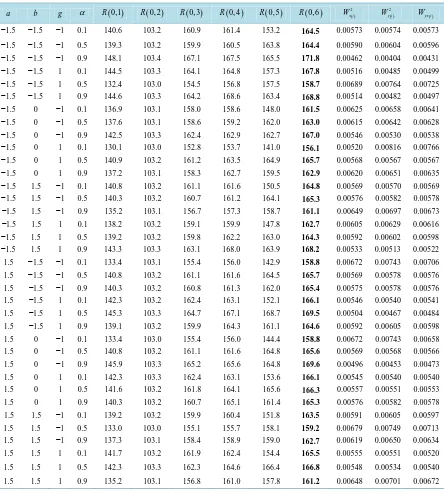
[image:8.595.92.536.230.722.2]

W are obtained through this simulation and are represented in the last three columns of Table 1.

Table 1. PREs of proposed class of estimators through simulation. a b g α R( )0,1 R( )0, 2 R( )0, 3 R( )0, 4 R( )0, 5 R( )0, 6 2_{( )}

x i

W 2_{( )}

y i

W Wyx i_{( )}

−1.5 −1.5 −1 0.1 140.6 103.2 160.9 161.4 153.2 164.5 0.00573 0.00574 0.00573

−1.5 −1.5 −1 0.5 139.3 103.2 159.9 160.5 163.8 164.4 0.00590 0.00604 0.00596

−1.5 −1.5 −1 0.9 148.1 103.4 167.1 167.5 165.5 171.8 0.00462 0.00404 0.00431

−1.5 −1.5 1 0.1 144.5 103.3 164.1 164.8 157.3 167.8 0.00516 0.00485 0.00499

−1.5 −1.5 1 0.5 132.4 103.0 154.5 156.8 157.5 158.7 0.00689 0.00764 0.00725

−1.5 −1.5 1 0.9 144.6 103.3 164.2 168.6 163.4 168.8 0.00514 0.00482 0.00497

−1.5 0 −1 0.1 136.9 103.1 158.0 158.6 148.0 161.5 0.00625 0.00658 0.00641

−1.5 0 −1 0.5 137.6 103.1 158.6 159.2 162.0 163.0 0.00615 0.00642 0.00628

−1.5 0 −1 0.9 142.5 103.3 162.4 162.9 162.7 167.0 0.00546 0.00530 0.00538

−1.5 0 1 0.1 130.1 103.0 152.8 153.7 141.0 156.1 0.00520 0.00816 0.00766

−1.5 0 1 0.5 140.9 103.2 161.2 163.5 164.9 165.7 0.00568 0.00567 0.00567

−1.5 0 1 0.9 137.2 103.1 158.3 162.7 159.5 162.9 0.00620 0.00651 0.00635

−1.5 1.5 −1 0.1 140.8 103.2 161.1 161.6 150.5 164.8 0.00569 0.00570 0.00569

−1.5 1.5 −1 0.5 140.3 103.2 160.7 161.2 164.1 165.3 0.00576 0.00582 0.00578

−1.5 1.5 −1 0.9 135.2 103.1 156.7 157.3 158.7 161.1 0.00649 0.00697 0.00673

−1.5 1.5 1 0.1 138.2 103.2 159.1 159.9 147.8 162.7 0.00605 0.00629 0.00616

−1.5 1.5 1 0.5 139.2 103.2 159.8 162.2 163.0 164.3 0.00592 0.00602 0.00598

−1.5 1.5 1 0.9 143.3 103.3 163.1 168.0 163.9 168.2 0.00533 0.00513 0.00522

1.5 −1.5 −1 0.1 133.4 103.1 155.4 156.0 142.9 158.8 0.00672 0.00743 0.00706

1.5 −1.5 −1 0.5 140.8 103.2 161.1 161.6 164.5 165.7 0.00569 0.00578 0.00576

1.5 −1.5 −1 0.9 140.3 103.2 160.8 161.3 162.0 165.4 0.00575 0.00578 0.00576

1.5 −1.5 1 0.1 142.3 103.2 162.4 163.1 152.1 166.1 0.00546 0.00540 0.00541

1.5 −1.5 1 0.5 145.3 103.3 164.7 167.1 168.7 169.5 0.00504 0.00467 0.00484

1.5 −1.5 1 0.9 139.1 103.2 159.9 164.3 161.1 164.6 0.00592 0.00605 0.00598

1.5 0 −1 0.1 133.4 103.0 155.4 156.0 144.4 158.8 0.00672 0.00743 0.00658

1.5 0 −1 0.5 140.8 103.2 161.1 161.6 164.8 165.6 0.00569 0.00568 0.00566

1.5 0 −1 0.9 145.9 103.3 165.2 165.6 164.8 169.6 0.00496 0.00453 0.00473

1.5 0 1 0.1 142.3 103.3 162.4 163.1 153.6 166.1 0.00545 0.00540 0.00540

1.5 0 1 0.5 141.6 103.2 161.8 164.1 165.6 166.3 0.00557 0.00551 0.00553

1.5 0 1 0.9 140.3 103.2 160.7 165.1 161.4 165.3 0.00576 0.00582 0.00578

1.5 1.5 −1 0.1 139.2 103.2 159.9 160.4 151.8 163.5 0.00591 0.00605 0.00597

1.5 1.5 −1 0.5 133.0 103.0 155.1 155.7 158.1 159.2 0.00679 0.00749 0.00713

1.5 1.5 −1 0.9 137.3 103.1 158.4 158.9 159.0 162.7 0.00619 0.00650 0.00634

1.5 1.5 1 0.1 141.7 103.2 161.9 162.4 154.4 165.5 0.00555 0.00551 0.00520

1.5 1.5 1 0.5 142.3 103.3 162.3 164.6 166.4 166.8 0.00548 0.00534 0.00540

We investigate the percentage relative efficiency (PRE) of ratio estimator yrRSS =θˆ1 (say), the Searls estimator ysRSS =θˆ2, the difference estimator ydRSS =θˆ3, [1] estimator yS RSS( ) =θˆ4 when λ λ1+ 2 ≠1 with respect to conventional estimator yRSS =θˆ0 (say). We also calculate PRE of the proposed class of estimators, say, yL RSS_{( )}1 =θˆ5 when

(

k1+k2=1

)

and when

(

k1+k2≠1

)

, say, yL RSS( )2=θˆ6, with respect to yRSS=θˆ0. The PRE of our proposed estimator and other existing estimators ˆθj, j=1, 2,, 6, with respect to con-

ventional estimator yRSS =θˆ0, is defined as

(

)

( )

_{( )}

0 0

ˆ

ˆ_,ˆ _{100, 1, 2, , 6.}

ˆ

j

j

MSE

PRE j

MSE

θ θ θ

θ

= × =  (27)

The PREs of our proposed estimator and other existing estimators with respect to conventional estimator are given in Table 1.

6. Conclusions

Since a b g, , and α are the fixed constants in [1] estimator and in the proposed class of estimators. There can be a large number of combinations for different values of these constants. Here, only limited number of results are reported in Table 1. Obviously, it can be observed through the simulation study in Table 1, that the proposed class of estimators is more efficient than all considered estimators. Its PRE increases from 164.5 to 171.8 when α changes from 0.1 to 0.9 but decreases slightly when α is close to 0.5. Generally, we can say

PRE of proposed class increases as value of α increases for fixed values of constants a, b and g[1]. Class of estimators has maximum PRE 167.5, but it is less efficient as compared to the proposed class of estimators for all the choices of constants reported in Table 1. Also from the Table 1, we can see that other competitor estimators are also less efficient than the proposed class of estimators. If we make comparison between the two proposed cases then the class of estimators in Case 2

(

k1+k2≠1

)

is more precise than the Case 1

(

k1+k2=1

)

. We can see from Table 1 that by fixing the values of a and b at −1.5, the proposed classes of

estimators give more precise results when the value of α is away form

0.5

, either close to 0 or 1. While by fixing positive values of the constants a and b, we get more precise results for α close to 0.5.

Therefore, the proposed class of estimators can be preferred over its competitive estimators in application under RSS.

Acknowledgements

The authors wish to thank the editor and the anonymous referees for their suggestions which led to improvement in the earlier version of the manuscript.

References

[1] Singh, H.P., Tailor, R. and Singh, S. (2014) General Procedure for Estimating the Population Mean Using Ranked Set Sampling. Journal of Statistical Computation and Simulation, 84, 931-945.

http://dx.doi.org/10.1080/00949655.2012.733395

[2] Mclntyre, G. (1952) A Method for Unbiased Selective Sampling, Using Ranked Sets. Crop and Pasture Science, 3, 385-390. http://dx.doi.org/10.1071/AR9520385

[3] Takahasi, K. and Wakimoto, K. (1968) On Unbiased Estimates of the Population Mean Based on the Sample Stratified by Means of Ordering. Annals of the Institute of Statistical Mathematics, 20, 1-31.

http://dx.doi.org/10.1007/BF02911622

[4] Samawi, H.M. and Muttlak, M.A. (1996) Estimation of Ratio Using Ranked Set Sampling. Biometrical Journal, 38, 753-764. http://dx.doi.org/10.1002/bimj.4710380616

[5] Dell, T. and Clutter, J. (1972) Ranked Set Sampling Theory with Order Statistics Background. Biometrics, 545-555. http://dx.doi.org/10.2307/2556166

[6] Stokes, S.L. (1977) Ranked Set Sampling with Concomitant Variables. Communication in Statistics: Theory and Me-thods, 6, 1207-1211. http://dx.doi.org/10.1080/03610927708827563

[7] Khan, L. and Shabbir, J. (2015) A Class of Hartley-Ross Type Unbiased Estimators for Population Mean Using Ranked Set Sampling. Hacettepe Journal of Mathematics and Statistics.

[8] Khan, L. and Shabbir, J. (2016) Hartley-Ross Type Unbiased Estimators Using Ranked Set Sampling and Stratified Ranked Set Sampling. North Carolina Journal of Mathematics and Statistics, 2, 10-22.

[9] Kadilar, C., Unyazici, Y. and Cingi, H. (2009) Ratio Estimator for the Population Mean Using Ranked Set Sampling. Statistical Papers, 50, 301-309. http://dx.doi.org/10.1007/s00362-007-0079-y

[10] Arnold, B.C., Balakrishnan, N. and Nagaraja, H.N. (2012)A First Course in Order Statistics. Vol. 54, Siam.

[11] Searls, D.T. (1964) The Utilization of a Known Coefficient of Variation in the Estimation Procedure. Journal of the American Statistical Association, 59, 1225-1226. http://dx.doi.org/10.1080/01621459.1964.10480765

[12] Khoshnevisan, M., Singh, R., Chauhan, P., Sawan, N. and Smarandache, F. (2007) A General Family of Estimators for Estimating Population Mean Using Known Value of Some Population Parameter(s). Far East Journal of Theoretical Statistics, 22, 181-191.

[13] Lohr, S. (1999)Sampling: Design and Analysis. Duxbury Press, Boston.

[image:10.595.90.534.287.634.2]

Appendix

Table A1. Some special cases of the proposed class of estimators.

1

k k2 α a b Estimator Remarks

1 0 0 0 1 ys RSS( )=y[ ]rss Usual RSS mean estimator

1 0 0 1 0 ( ) [ ]

( )

r RSS rss rss X

y y

x

 

 

= _{ }

  Usual RSS ratio estimaotr

λ 0 0 1 0 ( ) [ ]

( )

sr RSS rss rss X

y y

x λ  

= _{ }

 

Kadilar et al. (2009) ratio type estimator

1 β 0 0 1 yreg RSS( )=y[ ]rss+β

(

X−x( )rss

)

 Regression type estimator

1 k2 0 0 1 yd RSS( )=y[ ]rss +k2

(

X−x( )rss

)

 Difference type estimator

1 k2 0 1 0 ( ) [ ]

(

( )

)

( )

2

=

dr RSS rss rss rss X

y y k X x

x

 

 + −   

  _ _ Difference-ratio estimator

1

k k2 0 1 0 ( ) [ ]

(

( )

)

( )

1 2

gdr RSS rss rss rss X

y k y k X x

x

 

   

=_ + − _{  }

 

Generalied difference-ratio estimator

1 β 0 1 0 ( ) [ ]

(

( )

)

( )

regr RSS rss rss rss X

y y X x

x

β  

   

=_ + − _{  }

  Regression-ratio estimator

1 0 1 1 0 ( ) [ ] ( )

( )

exp rss

e RSS rss

rss X x

y y

X x

 − 

 

= _{ }

+

  Exponential type estimator

1 β 1 1 0 ( ) [ ]

(

( )

)

( )

( )

exp rss

rege RSS rss rss

rss X x

y y X x

X x

β  − 

   

=_ + − _{  }

+

 