Design of the Quantization Matrix in the Distributed Compressed Sensing Video Coding*

http://dx.doi.org/10.4236/jcc.2016.45003

How to cite this paper: Dai, Y.Y., Rui, X.H. and Zhao, X.Y. (2016) Design of the Quantization Matrix in the Distributed Com-pressed Sensing Video Coding. Journal of Computer and Communications, 4, 16-23.

http://dx.doi.org/10.4236/jcc.2016.45003

Design of the Quantization Matrix

in the Distributed Compressed

Sensing Video Coding

*

Yueyue Dai

, Xinhua Rui

, Xuanyu Zhao

1_{College of Telecommunications and Information Engineering, Nanjing University of Posts and}

Telecommunications, Nanjing, China

2_{School of Electric Power Engineering, Nanjing Institute of Technology, Nanjing, China} 3_{Nanjing Foreign Language School, Nanjing, China}

Received 29 February 2016; accepted 19 May 2016; published 26 May 2016

Abstract

In the frame of compressed sensing distributed video coding, the design of the quantization matrix directly affects the reconstruction quality of the receiving terminal of the video. In this article, we present a new design method of the Gaussian quantization matrix adapting to the compressed sensing coding, for that the distribution of the parameters of the image is featured of the characte-ristic of approximately normal distribution after measured by compressive sensing. By this way, the parameters of a certain quantity of the image frames depending on the video sequences gen-erated by the Gaussian quantization matrix possess certain adaptive capacity. By comparison with the plan of the traditional quantization, the quantization matrix presented in this article would improve the reconstruction quality of the video.

Keywords

Compressed Sensing, Distributed Video Coding, Gaussian Quantization Matrix

1. Introduction

With the increasingly complex and changeable monitoring environment, the simple data obtained by the tradi-tional wireless sensor networks does not meet the complete need of the people for monitoring the environment. For achieving the accurate monitoring of the environmental information, it is an active demand that we intro-duce the media of the image, audio and video with abundant information into the environment monitoring activ-ities based on the sensor networks. in this context, the wireless multimedia sensor networks emerge as the times require [1]. In the wireless multimedia sensor networks, the technology of the traditional video coding does not meet the low complexity requirement of the wireless multimedia sensor networks for the nodes. The traditional

*_{This work is financially supported by NSFC Projects No. 61471162, NSF of Jiangsu Province (BK20141389), and Innovation Project of}

video coding plan using the technology of “Joint Coding, Joint Decoding” [2]. This technology have a very high compression efficiency, but it is very sensitive to the channel error. The error propagation happens easily under the situation for the high rate of channel error. It leads to an unsatisfactory result of the effect of reconstruction the images [3]. For resolving this issue, the researcher considered a method composed of data collection and compression totally different from the traditional collection method base on Nyquist Rate, which is the com-pressed sensing.

The theory of the compressed sensing is a new theory of the new signal processing presented by Z. X. Tao, Donoho, et al. in the year of 2006 [4]. It broke the bottleneck of the Nyquist Theorem. It combines the collection and the compression and uses the optimization algorithm reconstruction at the collecting terminal. It is featured on the advantage of simple coding and strong capacity of anti-errors. It does meet the requirement of the wire-less multimedia sensor networks. In the recent years, in the wirewire-less multimedia networks, the theory of the compressed sensing has been applied to the distributed video coding. For example, the WINES Laboratory leaded by Professor T. Melodia of New York Buffalo devotes themselves to the research of the video coding transmission plan based on the compressed sensing under the wireless multimedia sensor networks [5], and they have already gained a lot of achievements.

2. Relative Basic Theory

2.1. Compressed Sensing

The Compressed Sensing theory broke the bottle neck of the Nyquist Sampling Theorem. It combines the processing of the sampling and compression, and uses the non-adaptive linear projection for maintaining the original structure of the image signal, and can rebuild effectively the image signals by the optimization algo-rithm at the receiving terminal. In the compressed sensing theory, the image is represented as the vector _x∈RN

and the length of the vector is represented as N. The reversible transformation matrix ψ of N*N exists hypo-thetically. It meets

x= ∗

ψ

In this equation, s is the K-sparse vector, that is S₀ =K and K < N. .

p represents that is the norm of p.

It means that transform the image by a certain transformation into certain field could be sparse, for example, wavelet transform. Then, M measuring values are taken out from N values of x. It is required that M < N. This step is achieved by the measuring matrix φ as follows.

*

y=φ x (2)

* *

y=φ x=φψ s= Φ ∗s (3)

After receiving y at the receiving terminal, the x needs to be recovered. As M < N, the system is underdeter-mined, that means it is countless solutions. If a solution s0 meets the Equation (3), the vector _s* = +_s0 _{n (the} n represents the empty matrix of the same size as s0), it also meets the Equation (3). By the proof of the theory, if the measuring matrix φ and the transformation matrix ψ are uncorrelated, and the sparsity K is smaller than the specified threshold, we can get the s which meet the requirements by the most sparse solution of the Equation (3). The most sparse solution corresponds to the y of the receiving terminal. It is a NP-hard problem [6]. There is always the sparsest solution for the matrix φ and this solution is sole. It equals to the following equation:

1

min s s t. . y− Φ <s

ε

In this equation, ε is the smallest threshold. Thus, the problem is transformed to an optimal solution prob-lem. By the transformation matrix ψ , and both of the measuring matrix φ and the received y can be pro-ceeded the reconstruction of x [7].

2.2. DVC: Distributed Video Coding

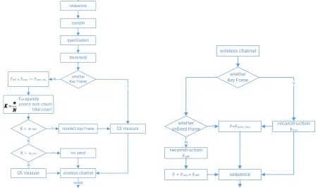
the video sequences and transform the complexity from the coding end to the decoding end. The characteristics of the Distributed Video Coding adapt well the requirements of the Wireless Multimedia Sensor Networks. The Distributed Video Coding has become the hottest research in the recent years. With the presentation of the Compressed Sensing Theory, D. Baron et al. introduced the compressed sensing theory into the distributed vid-eo coding and presented a completely new thvid-eory of signal processing, that is the Distributed Compressive Vid-eo Sensing [9]. The research of this article is based on the frame of the distributed compressive sensing as Fig-ure 1.

The research of the distributed compressive sensing is divided into the research of the sparse representation algorithm of the coding end, the research of the reconstruction algorithm of the decoding end and the research of the transmission strategy in the transmission process. We don’t consider the influence of the sparse representa-tion algorithm and the reconstrucrepresenta-tion algorithm in this article. We study the influence of the quantizarepresenta-tion method in this article and design and achieve the new quantization matrix adapting to the distributed compressive sens-ing video codsens-ing.

3. Gaussian Quantization Matrix

3.1. Distribution of the Measuring Coefficient of the Compressed Sensing

The design of the quantizer is vital in the transmission system. A good quantizer can improve effectively the re-construction quality at the coding end. We will present a new Gaussian quantization matrix base on the com-pressed sensing distributed video coding in this section.

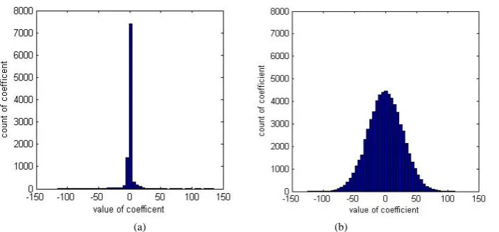
In the previous studies, different standard of video coding corresponds the different design of the quantization matrix. For example, in the first image of the announcer video sequences, under the MEPG standard, the distri-bution of the coefficient after discrete cosine transform can be seen as Figure 2(a). The distridistri-bution of the coef-ficient of the image concentrate mainly in the low frequency region in Figure 2(a), so the design of the quanti-zation matrix follows also the standard of small quantiquanti-zation step in the low frequency region and big quantiza-tion step in the high frequency region, that is the dense quantizaquantiza-tion in the low frequency region and the sparse quantization in the high frequency region [10]. This is also conforming to the theoretical basis of vision of

sequence input sample quantization threshold whether Key Frame CS measure Fdiff = Fnow — Fprev_key

Fdiff sparsity

unzero num count total count

K > αhigh N

Y

reselect Key Frame Y

CS measure wireless channel

output

K > αlow N N no send Y wireless channel whether Key Frame reconstruction Fkey reconstruction Fdiff Y

F = Fkey + Fdiff

whether

unSend Frame Y F=Fprev_key

N

sequence

(a) (b)

Figure 2. Histogram of the distribution of the parameters. (a) DCT parameters; (b) CS measuring

parameters.

human eyes as the vision of human eyes isn’t sensitive to the errors of the high frequency part while is sensitive to the low frequency part.

The idea of the compressed sensing is that the sparse matrix in a certain projection domain is transformed to another one projection domain and the sparsity of the matrix is increased, therefore it plays the role of signal compression. The distribution of the image coefficients after measuring by the compressed sensing can be known from Figure 2(b). Comparing with the distribution Figure of the coefficients after the DCT (discrete co-sine transform), the parameters are also concentrated around the 0 and the large value data of both sides are very few. As we can see in Figure 2(b), the distribution of the parameters after the compressed sensing is the Gaus-sian distribution (normal distribution).

The distribution of the measuring coefficients of the compressed sensing refers to the histogram 2b.The dis-tribution of the image coefficients after compressed sensing is the Gaussian disdis-tribution. Meanwhile, as the cha-racteristic that the vision of human eyes isn’t sensitive to the high frequency error but sensitive to the low fre-quency error, if the design of the quantization matrix also follows the Gaussian distribution, the distribution of the coefficients of the quantization matrix is also the Gaussian distribution. The better quantization effect will be achieved by this kind of quantization matrix. We call it as the Gaussian Matrix in this article.

3.2. Design of Gaussian Quantization Matrix

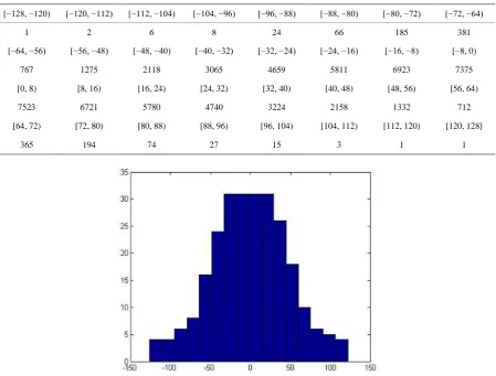
The Gaussian Quantization Matrix obtained by the characteristic of the distribution of the coefficients after the measuring of the image. The distribution of the coefficients of the quantization matrix depends on the distribu-tion ratio of the coefficients after measuring. The coefficients of the first image of the announcer video se-quences after measuring is presented through the histogram in Figure 2(b). Before measuring the image coeffi-cients, we proceed the operation of reducing the mean from all of the coefficients in order to increase the sparsi-ty. The distribution of the coefficients of Figure 2(b) is visualized and the parameters are showed quantitatively in Table 1.

The Gaussian Quantization Matrix designed in this article, the distribution of the quantitative coefficients also follows the specific gravity distribution of the image coefficients. As we can observe from the data in Table 1, the part nearby the 0 is in the dense quantization and the part far away from 0 is in the sparse quantization. We define this distribution function similar to the Gaussians as

( )

nearGaussian x =count count (5)

So we can’t run a too crude quantization for the big value data. The solution is to run a certain degree of uplift for the Gaussian distribution function. Uplift the Gaussian distribution according to the Equation (6).

( )

( )

Q=nearGaussian x +mean x (6)

We add the average value of the coefficients of the previous image to the standard Gaussian distribution and change effectively the distribution of the quantization coefficients by this way. The quantization matrix can be obtained by programming after understanding the distribution of the quantization coefficients. The histogram of the distribution of the quantization matrix is presented in Figure 3 through the quantization matrix obtained in the distribution of the image coefficients. The matching effect of the distribution of the quantization coefficients and the measuring coefficients in the histogram is very good. The effect of the quantization matrix can be veri-fied by the subsequent experimental simulations.

4. Comparison of the Effects

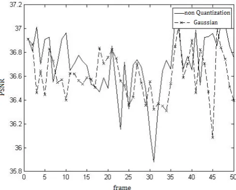
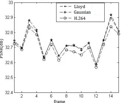
We analyze the experimental simulation of the Akiyo video sequences in this article. From the comparisons of the reconstruction effect of 3 kinds of quantitative methods in Figure 4 & Figure 5, we can know that the re-construction effect is the best when we don’t make any quantization for the video sequences. Apparently, the quantitative error won’t be introduced if we don’t make any quantization, and the high accuracy of the data can be ensured, therefore, the high quality of the reconstruction can be assured. However, the quantity of the image data will not be compressed if we don’t make any quantization, and the high accuracy of the data will become the encumbrance of the transmission and the reconstruction processing, so the time consumption of the method of non-quantization is the longest.

Table 1. Distribution of the coefficients after measuring the compressed sensing of the image.

[−128, −120) [−120, −112) [−112, −104) [−104, −96) [−96, −88) [−88, −80) [−80, −72) [−72, −64)

1 2 6 8 24 66 185 381

[−64, −56) [−56, −48) [−48, −40) [−40, −32) [−32, −24) [−24, −16) [−16, −8) [−8, 0)

767 1275 2118 3065 4659 5811 6923 7375

[0, 8) [8, 16) [16, 24) [24, 32) [32, 40) [40, 48) [48, 56) [56, 64)

7523 6721 5780 4740 3224 2158 1332 712

[64, 72) [72, 80) [80, 88) [88, 96) [96, 104) [104, 112) [112, 120) [120, 128]

365 194 74 27 15 3 1 1

Figure 4. Comparison of uniform and Gaussian quantization.

Figure 5. Comparison of Gaussian non Gaussian quantization.

Figure 6. H.264 comparison of the effects of the standard quantization, Lloyd quantization and the Gaussian quantization.

Table 2. Table of time consumption of the generations of the Gaussian

quan-tization matrix and the Lloyd quanquan-tization matrix.

Quantization type Consuming time (s)

Gaussian quantization matrix 0.1851s

Lloyd quantization matrix 1.8034s

As we can see from Table 2, the time consumption of the generation of Gaussian Quantization Matrix is 0.1851 s, and the time consumption of the generation of the Lloyd Quantization Matrix is 1.8034 s and it is al-most 10 times of that of Gaussian Quantization Matrix. Under the situation of the approximative effects, the time consumption of the generation of the Gaussian Quantization Matrix is only one tenth of that of the Lloyd Quantization Matrix.

5. Conclusion

In this article, we analyze the characteristics that the distribution of the image coefficients is as the Gaussian Distribution and the distribution of the quantization matrix coefficients of the Gaussian Quantization Matrix is also the Gaussian Distribution under the distributed compressive sensing video coding, and then make the com-parison with the Uniform Quantization, and finally, we got the conclusion that the effect of the new quantization matrix is better. The effect of the Gaussian Quantization is not as good as that of the non-quantization method, however, from the point of the efficiency, the time consumption of the Gaussian Quantization Matrix is much smaller than that of the non-quantization method. The time consumptions of the Gaussian Quantization and the Uniform Quantization are the same as the quantization parameters and the quantization matrix of these 2 kinds of quantization matrix are the same. By such comparison, we can achieve the conclusion that both of the effect and the efficiency of the Gaussian Quantization Matrix are better.

References

[1] Sharif, A., Potdar, V. and Chang, E. (2009) Wireless Multimedia Sensor Network Technology: A Survey. Proceedings of 7thIEEEInternationalConferenceonIndustrialInformatics, June 2009, 606-613.

http://dx.doi.org/10.1109/indin.2009.5195872

[2] Kang, L.-W. and Lu, C.-S. (2009) Distributed Compressive Video Sensing. ProceedingsofIEEEInt.Conf.on Acous-tics, SpeechandSignalProcessing (ICASSP), April 2009, 1169-1172. http://dx.doi.org/10.1109/icassp.2009.4959797

[3] Chen, R., Wu, M.H. and Tong, Y. (2013) Feedback-Free Wavelet Based Distributed Coding for Video. Sensors & Transducers, 153, 192-199.

http://dx.doi.org/10.1109/TIT.2006.871582

[5] Melodia, T. and Pudlewski, S. (2009) A Case for Compressive Video Streaming in Wireless Multimedia Sensor Net-works. IEEECOMSOCMMTCE-Letter, 4, 46-48.

[6] Lebedeff, D., Mathieu, P., Barlaud, E., Lambert-Nebout, C. and Bellemain, P. (1995) Adaptive Vector Quantization for Raw SAR Data. ProceedingsofAcoustics, SpeechandSignalProcessing, 4, 2511-2514.

http://dx.doi.org/10.1109/icassp.1995.480059

[7] Fowler, J.E., Mun, S. and Tramel, E.W. (2012) Block-Based Compressed Sensing of Images and Video. Foundations andTrendsinSignalProcessing, 4, 297-416. http://dx.doi.org/10.1561/2000000033

[8] Girod, B., Aaron, A., Rane, S. and Rebollo-Monedero, D. (2005) Distributed Video Coding. ProceedingsoftheIEEE,

93, 71-83. http://dx.doi.org/10.1109/JPROC.2004.839619

[9] Baron, D., Duarte, M.F., Wakin, M.B., Sarvotham, S. and Baraniuk, R.G. (2009) Distributed Compressive Sensing.

IEEETransactionsonInformationTheory, 55, 12-53.