Estimating SUR Tobit Model while errors are gaussian scale mixtures: with an application to high frequency financial data

Munich Personal RePEc Archive

Estimating SUR Tobit Model while

Errors are Gaussian Scale Mixtures: with

an Application to High Frequency

Financial Data

Qian, Hang

Iowa State University

July 2009

Online at

https://mpra.ub.uni-muenchen.de/31509/

Estimating SUR Tobit Model while Errors are Gaussian Scale Mixtures

––

with an Application to High Frequency Financial Data

Hang Qian

Iowa State University

Abstract

This paper examines multivariate Tobit system with Scale mixture disturbances. Three estimation methods, namely Maximum Simulated Likelihood, Expectation Maximization Algorithm and Bayesian MCMC simulators, are proposed and compared via generated data experiments. The chief finding is that Bayesian approach outperforms others in terms of accuracy, speed and stability. The proposed model is also applied to a real data set and study the high frequency price and trading volume dynamics. The empirical results confirm the information contents of historical price, lending support to the usefulness of technical analysis. In addition, the scale mixture model is also extended to sample selection SUR Tobit and finite Gaussian regime mixtures.

1. Introduction

The seminal work of Amemiya (1974) inspired a variety of research on Seemingly Unrelated Tobit Regression (SUR Tobit) model. Since its advent, SUR Tobit model has been firmly integrated with economic theory where corner solution prevails due to non-negativity constraints, capacity limits or government regulations. Wales and Woodland (1983) derived the censored demand systems based on Kuhn-Tucker conditions. Lee and Pitt (1986) adopted dual approach to the demand system using virtual price in place of complementary slackness conditions. Those models per se are elegant; the remaining difficulties are largely computational – likelihood function entails evaluations of multiple integrals without analytical solution.

Recent years witness increasing popularity of SUR Tobit model in applied micro-econometric studies. The driving force is apparently the advance of numerical methods and computation resources. Broadly speaking, there are four common methods to estimate the SUR Tobit system, namely Maximum Simulated Likelihood (MSL), Heckman Two Steps, Expectation-Maximization (EM) algorithm and Bayesian Posterior Simulator.

Borsch-Supan and Hajivassiliou, 1993; Keane, 1994) was used to evaluate the integral. Kao et.al (2001) also adopted that simulator to study a seven-goods linear expenditure demand system.

Secondly, the two step procedure offers a less computational alternative to MSL. Nowadays, it becomes clear that the Heien and Wessells (1990)’s two step procedure suffers from internal inconsistency, but their ideas do set the seeds for Shonkwiler and Yen (1999) modification. Su and Yen (2000) applied that procedure to study censored system of cigarette and alcohol consumption.

Thirdly, E-M algorithm can be suitably applied to SUR Tobit model, offering a consistent and asymptotically efficient estimator. Huang et.al (1987) provides analytical formulae for the E-step and M-step in the two-dimension censoring system. Another author Huang (1999) extended it to the multiple-equation case by Monte Carlo E-step plus conditional M-step.

Fourthly, Bayesian posterior simulator competes with the traditional ML based point estimator. Chib and Greenberg (1995, 1998) examined limited dependent variable model in the Bayesian SUR framework. Essentially observable data are augmented by draws from their truncated conditional distribution whenever censoring occurs. To apply the Bayesian approach to the SUR Tobit, Huang (2001) outlined the MCMC steps to implement the simulation.

It should be noted that the main attraction of SUR Tobit system lies in its flexible correlation structure, induced by multivariate normally distributed disturbances. (On the other hand, this is the source of computational burden!) Admittedly, it is possible to circumvent the normal distribution by resorting to GEV specification (e.g. Pudney, 1989), error component structure (Butler and Moffitt,1982), Copula approach (e.g. Yen and Lin, 2008 used Frank’s copula with log-Burr marginals), etc, we do not want to impose stringent restrictions on disturbance terms, but rather lessen it by introducing mixture models, which admit normality as a special case. It turns out that our methods are still computationally tractable.

In the main text, we will discuss the estimation of SUR Tobit model with Gaussian scale-mixture disturbances. In microeconomics, individual unobserved heterogeneity might justify the varied error variance. In finance, it is well documented that security prices always exhibit leptokurtosis and/or skewness (e.g. Fama,1965; Praetz, 1972; Peiro, 1994, to name a few). Investors usually feel the stock prices crawling upwards for months and plummet in a day. The magnitude of crash on Black Monday of 1987 is hard to reconcile with the relative thin tail of normal distribution. It is common for high-frequent financial data exhibiting asymmetry, leptokurtosis and extreme value. Gaussian scale-mixture has a marginal distribution as multivariate t, thus is able to accommodate leptokurtosis. Of course, there are other tractable mixtures to model departure from normality, such as finite Gaussian regime mixtures, skewed normal, which could capture skewness as well. We will briefly discuss some extensions at the end of the paper.

The focus of the paper is on the various estimation methods for the SUR Tobit model with mixture errors. Treating the unobserved heterogeneity as an additional latent variable, we develop three methods to estimate the model: MSL, EM and Bayesian posterior sampler. Comparisons of the three methods are investigated through artificial data set with known DGP. We also illustrate our approach by studying the price and volume interactions using high-frequency trading data of financial derivatives, where non-trading accounts for a non-negligible portion of the data.

2. Estimation Methods

2.1 The model

The linear regression form of SUR Tobit with Gaussian scale-mixtures can be written as:

, ( ) , ( ) ……

, ( )

| ( ) , where is m*m positive definite matrix . /

For future reference, stack the variables in the obvious way,

(

+ , (

+ , ( ) , (

+ , (

+

( + , ( + , ( + , ( +

The latent variables and are not observable. The goal of statistical inference is to estimate the parameter from the data and . Notice that in the model, conditional on latent scale , is multivariate normal ( ). For tractability, the latent scale has an inverted Gamma distribution

. / so that ‘s marginal distribution is multivariate t ( ) (See Appendix A1).

It is true that in some applications, researchers might encounter models more complicated than the

above setup. For instance, Wales and Woodland (1983)’s Kuhn-Tucker model does not have a regression form, could be intertwined with and so that the system is non-linear. In some other applications, say Su and Yen (2000), the determination of individual participation and activity level are separated. However, the estimation methods outlined below can be adapted and easily extended to non-linearity and sample selection models.

Compared with single-equation Tobit, the multivariate system might have various patterns of censoring. To be more exact, an m-variate system has patterns ranging from no censoring to all censorings. Without loss of generality, for some individual t, rearrange the order of variables so that the first dependent variables are intact but the last variates are censored to zero. We use the

subscript “u” to denote the non-censored block, and subscript “c” to denote the censored block. (The special cases and correspond to no censoring and all censoring respectively. For notational simplicity, treat the former as an empty “c” block, and the latter as an empty “u” block.)

For some individual t, the variables are partitioned to be:

(

* , (

* , (

* , ( * , (

The partition is useful since in all the three methods discussed below, distribution of censored block, conditional on the knowledge of uncensored block, will be intensively explored. It should be noted that the conditional distribution of MVN variates (blocks) are still normal, while that of MVT do not have a familiar form. Therefore, the inclusion of latent scale bridges the flexible MVT and the tractable MVN.

2.2 Maximum Simulated Likelihood

Full information maximum likelihood is the most straightforward way (at least conceptually) to estimate the above system, provided that the dimension is not too high. It counts the contribution of censored probability plus that of uncensored density. Fishy at the first glance, the blending likelihood has been shown by Amemiya (1973) to be valid. Schnedler (2005) further established rules to construct likelihood for more general censoring problems. The maximizer is proven to be root-N consistent, asymptotically efficient and normally distributed under regularity conditions.

In our model, the log likelihood is ∑ ( ) , where

( ) ∫ ∫ ( )

( ) ∫ ∫ ( | ) ( | )

To avoid confusion, the variables and the intervals have the order like ∫ ∫ ( )

It can be shown that (see Appendix A2)

( )

| { 0 ( ) ( )1

}

| [ ( ) ( ) ]

The crux of ML estimation is to calculate ∫ ∫ ( | ) ( | )

, which belongs to the c.d.f of the “multivariate generalized t-distributions family” (Arslan, 2004), with probability evaluated at rectangular region ( ) for each element. The integral does not have a close-form solution. For lower dimension case, Gaussian quadrature might provide a faster and more accurate solution, but simulation techniques must be employed for higher dimensional problems.

Nowadays, GHK simulator (Geweke, 1991; Borsch-Supan and Hajivassiliou, 1993; Keane, 1994) is a popular choice for evaluating probabilities of multivariate normal distribution. Hajivassiliou et al. (1996) reviewed many available simulators and concluded that GHK simulator outperforms others.

In this paper, we extend GHK simulator to evaluate multivariate t family c.d.f.. It turns out that only one more layer need to be added to the recursive conditionings. That is, we first obtain a draw from IG distribution and then start the usual GHK recursive truncated normal draws, and finally calculate a series of univarite normal c.d.f.s.

The details are as follows.

We want to calculate ( )

Cholesky decompose the covariance matrix , denote

(

)

Define ( ) so that | ( )

By change of variables, it is easy to show

( ) ∫ ∫ ∫ ( ) ( )

, ( ) ( )

-where

√ ,

√ √ , …,

√ ( ) √

, are i th element of

( ) is expectation w.r.t. . /

( ) is expectation w.r.t. ₍ ) ( ) … …

( ) is expectation w.r.t. ₍ ) ( )

So the GHK simulator adapted to MVT c.d.f has the following algorithm

i) Generate a draw . /

ii) Conditional on , recursively generate draws , … , iii) Calculate ( ) ( )

iv) Repeat i) - iii), and take the average of results of iii), which approximates ( )

To apply the above simulator to our problem, we simply need to modify step i) by replacing the

standard . / with the posterior { 0 ( ) ( )1 }

2.3 Expectation-Maximization Algorithm

In their influential paper, Dempster et.al (1977) proposed an intuitive and insightful method to estimate the latent variables model. The basic idea of E-M algorithm is that if the latent variables were known, the complete data likelihood would be much easier to maximize, usually with close-form solution. To address the unknown, we take the expectation of complete data likelihood w.r.t. the posterior distribution of latent variables (conditional on our latest estimated parameters). E-M algorithm can be viewed as lower bound optimization, and each round of E-step and M-step will lead to an updated estimator. The beauty of the approach is that the likelihood will never decrease in iteration and will converge to the maxima under fairly weak regularity conditions.

and Meyer(1953) , Tallis(1960) did provide the formulae, which, unfortunately, involve a series of cumbersome MVN c.d.f. As is known, the robust E-M algorithm comes with the price of slow convergence. It usually takes hundreds of iterations before convergence is achieved. If dozens of c.d.f. are calculated in each iteration, it would take very long time to implement the algorithm. In this paper, we extend

Huang(1999)’s algorithm featuring Monte Carlo E-step plus conditional M-step. In our model, there are two latent variables— and . Direct Monte Carlo E-step is not applicable, so we propose the MCMC to carry out the E-step.

The details of the algorithm are as follows:

The complete data log likelihood can be written as

( | )

∑ , ( | ) ( | ) ( )- ∑ ( | ) ( | )

∑ < . / . / . /

| | _{( ) ( )} =

We use the informal notation “constant” to represent those additive terms which do not interact with

model parameters , The rational is that our goal is to maximize the expected likelihood w.r.t.

where terms labeled as “constant” play no role. Note that some stand-alone functions of latent variables,

such as , can also be dumped.

To calculate the expectation of above likelihood, we first need to find out the posterior distribution of latent variables, i.e. | ( ) ( ) ( ) , where ( ( ) ( ) ( )) stands for estimators produced by latest round of iteration. (E-step must be implemented in that fashion, or the likelihood cannot be guaranteed to increase).

Unfortunately, the (joint) posterior distribution of do not belong to any recognizable family. That is to say, the posterior mean ( ) , ( ) , [ ( ) ( )] do not have a close form expression, let alone analytical expected likelihood. Simulations are needed to perform E-step.

Fortunately, the posterior conditional distributions do have a recognized form, so that Gibbs sampler can be employed to obtain posterior draws, which could be used to simulate expected likelihood.

For the time being (only in Section 2.3), define ( ) (

* , ( ) ( * , other notations

are same as Section 2.1

| ( ) ( ) ( ) ( )[ ( ) ( )] | ( ) ( ) ( ) ₈ ( ) ₀ ( )

( ( ))( ( ))

( ( )_{)1 9}

Note that the posterior conditionals of is truncated MVN. Geweke(1991) discussed sampling from univariate as well as multivariate truncated normal distribution. For truncated MVN, the distribution of one element conditional on other elements is univariate truncated normal, so that draws can be obtained via Gibbs sampler. In our case, an additional step, namely | , will be added to the Gibbs cycle to obtain

posterior draws { _{( ) ( )}}

, .

The expected complete data likelihood then can be approximated by the ergodic mean:

∑ ∑ < . / . / . / ( ) ( )

( ) | | ( ) ( ( ) ) ( ( ) ) =

Now that E-step has been done, M-step is on the way.

Note that even in SUR model, the likelihood function cannot be optimized analytically w.r.t. all at once. Here we are in the same position. Only if we maximize conditional on or optimize conditional on can we obtain close-form solutions. The conditional M-step still ensures the non-decreasing of likelihood as well as convergence. It is easy to show the updated estimators are: (See Appendix A3)

( ) _{0∑ . ∑}

( )

/

1

∑ 0 _{. ∑}

( )

( ) /1

( )

∑ ∑ 0 ( ) ( ( ) )( ( ) )1

( ) _{∑ 0 . / . / . / . ∑ ( )}

/ . ∑ ( ) /1

Intuitively, ( ) is a weighted OLS estimator by disturbance precisions, ( ) is the average of residual covariance matrix across equations. ( ) does not have a close-form, but the scalar can be easily optimize by Newton type numerical procedure, or even brute-force grid search!

2.4 Bayesian Posterior Simulator

E-M algorithm lies somewhere between the ML and Bayesian approach. On the one hand, E-M focus on the maximization of likelihood function and indeed obtain point estimators of . On the other hand, E-M also yields, as a by-product, the posterior distribution of the latent variables .

Bayesian approach treats the latent variable in the same manner as the parameters, and aims at joint posteriors of . Bayesian posterior simulator addresses the latent variables in the most intuitive way—simply take a random draw from its posterior distribution so as to augment the data.

Chib and Greenberg (1995, 1998) examined limited dependent variable model in the Bayesian SUR framework. Huang (2001) outlines the full set of conditionals for Gibbs sampler of SUR Tobit model. In our model with Gaussian scale-mixtures, only two additional steps will be added to the sampler—one is to take posterior draws for latent scale , the other is to sample degree of freedom parameter . The latter do not have a recognizable distribution, and therefore Metropolis-within-Gibbs procedure is employed to carry out MCMC. Compared with E-M algorithm outlined in the previous section, the posterior conditionals of latent variables are almost identical, but we need to specify the suitable priors to derive the posteriors of as well.

The proper priors are assumed to be:

( )

_{( )} ( )

The full set of posterior conditionals are: (See Appendix A4)

where [∑ ]

[∑

]

_{| 2 [ ∑ ( )( )}

] 3

| { 0 ( ) _{( )1 }}

| ( )[ ( ) ( )]

( | ) ∏ [ . / . / ] ( ) . /

( )

All posterior conditionals come from easy-to-draw distributions except for | , which does not have a recognizable form. Generally speaking, there are three ways to handle the case: one is to discretize the degree of freedom parameter (Albert and Chib, 1993). However, experience tells us that Gibbs sampler might perform poorly in the presence of discrete variates, since the chain usually move slowly across the parameter space. It is difficult to take a sudden leap to another discrete regime. Another approach is direct rejection sampling, but the supremum of the source and target density might be difficult to calculate in this case. Finally, the preferred approach is Metropolis-Hasting sampler within Gibbs. (In fact, Gibbs is a special case of M-H with acceptance probability of one). Here we use the normal random walk proposal, which performs satisfactorily.

3. Comparison of Estimators

In this section, we will apply the three estimation methods, namely Maximum simulated likelihood (ML hereafter), Expectation Maximization (EM hereafter), and Bayesian posterior simulators (BAY hereafter), to simulated data. The purpose of generated data experiment is twofold. First and foremost, despite the fact that they all yield consistent estimators, their finite sample properties are unknown (not applicable to Bayesian estimators, they are all finite sample in nature). Through generated data Monte Carlo experiments, we can compare their relative performance for a given sample size. Secondly, SUR Tobit model is easier said than done — practically computation poses the greatest challenge. Through the experiment, we attempt to find out the relatively economical way to estimate the model.

We will conduct two types of experiments. One is repeated experiments with fixed sample size of generated data, from which we can study the finite sample relative efficiency of varied estimators without resorting to asymptotics. The other is experiments with increasing sample size, so that we can learn the sensitivity of sample size to the performance of differed estimation methods.

Codes are run on an ordinary desktop computer (Pentium Dual 2.5GHZ / 3GB RAM / 64 bit Vista / Matlab 2009a). Computation time is recorded for reference purpose only, which obviously have much to do with the quality of the codes and the ability of the programmer.

As for the criteria of comparison, basically we compare the MSE of varied estimators. Since the researcher sets the DGP, the true parameter vector is known. Using one set of generated data, we obtain estimators ̂ , ̂ , and ̂ (posterior mean, by default). Repeat the process R times, we

obtain { ̂ ( )}

We first compare and report the regression coefficients one by one. Let , ̂ , ̂ , and ̂ be a corresponding element of the parameter vector , ̂ , ̂ , ̂ . We report the following:

Sample mean of estimators: ̂( ̂ ) ∑ ̂ _{( )}

Standard deviation of estimators: ̂( ̂ ) √ ∑ [ ̂ _{( )} ̂( ̂ )]

MSE of estimators: ( ̂ ) ∑ ( ̂ _{( )} )

E-M and Bayesian counterparts are defined in the same manner.

In addition, we also report some “composite indicators”. First of all, MSE matrixes are calculated:

( ̂ ) ∑ ( ̂ ( ) ) ( ̂ ( ) )

( ̂ ) ∑ ( ̂ ( ) ) ( ̂ ( ) )

( ̂ ) ∑ ( ̂ ( ) ) ( ̂ ( ) )

If, for example, ( ̂ ) ( ̂ ) is positive definite, then we conclude ̂ has a smaller MSE, thus is preferred to ̂

Since it is possible that the difference of MSE matrix is neither positive definite nor negative definite, (i.e. some of the eigenvalues are positive and others are negative, hence no conclusion), we report a scalar indicator “quadratic risk” as well, which always enables a ranking.

Quadratic risk:

( ̂ ) ∑ ( ̂ ( ) ) ( ̂ ( ) )

( ̂ ) ∑ ( ̂ ( ) ) ( ̂ ( ) )

( ̂ ) ∑ ( ̂ ( ) ) ( ̂ ( ) )

Estimator with smaller quadratic risk is preferable.

3.1 Repeated experiments with fixed sample size

The data generating process are as follows:

, ( ) , ( ) , ( ) , ( )

The true parameter values are set to be

(

, | [( , (

,] , . / ,

Regressors are drawn from standard normal.

The sample size is fixed at . For a given sample, three estimation methods are applied to the same data. Then generated data experiments are repeated for times (Due to limits of computation resources, repetition times are not very large. However, statistics obtained from each experiment are strictly iid, so it is still quite informative).

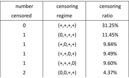
As is seen from Table 3.1.1, more than 68% of the data are subject to censoring, to some varied degree from one variable (40% of the data) to four variables (1% of the data). In the presence of non-negligible portion of censored data, use OLS or GLS to estimate the SUR system will cause inconsistency. Tobit-type approach must be used to explicitly account for censoring. This is confirmed by Table 3.3.2, which shows the native regression on the basis of equation-wise OLS and GLS. The results suggest that the estimators are severely biased downwards and the MSEs are huge.

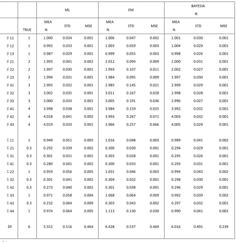
Table 3.1.3 to 2.2.5 compares the three consistent and asymptotically efficient estimators, namely ML, EM and Bayesian approach, in the context of given sample size T=2000. The major finding of the experiments is that Bayesian posterior simulators outperform any other estimators, unparalleled in terms of accuracy, stability and speed.

The accuracy of estimators can be compared by MSE of individual coefficients and the composite indictor such as quadratic risk. Though the mean of ML, EM and Bayesian estimators are all reasonably close to the true parameters, they differ substantially in MSE. The EM algorithm has the largest MSE, followed by ML estimators. Bayesian simulators has the least MSE in almost every individual coefficient. It is not because the EM algorithm itself is less accurate; the lack of preciseness is most likely induced by MCMC in the E-step. We only use 5000 draws to simulate the expected complete data likelihood, which could be less precise since MCMC draws are not independent. However, to choose 5000 draws is largely a practical concern—the fact is that every iteration entails such a simulation and EM algorithm usually takes hundreds of iterations to achieve convergence. It would be too costly to take larger number of draws.

A hidden factor affecting accuracy of estimators is starting values. For ML and EM, we use single equation Tobit with normal disturbances as the starting values, which are already reasonably close to the true parameter (but not consistent due to MVT errors). If we had picked the starting values at random, it could have been a disaster for ML and EM estimators. However, for Bayesian approach, we indeed picked the starting value at random, simply drawing from the prior, which can be far away from the true parameters. For example, degree of freedom is initially drawn from ( ). The beauty of Gibbs sampler is that convergence is guaranteed despite the starting value under regularity conditions of Markov Chain. Indeed people use dispersed starting value to test the convergence of the chain. From this perspective, the Bayesian simulator is superior. In our experiments, the number of draws is 30000 with the first 10% draws burned in. The posterior mean of simulators are quite close in every experiments—an informal evidence suggesting convergence of the Markov Chain.

asymptotic distribution simply because we set the DGP by ourselves. By repeating the experiments independently for many times, we simply calculate the sample standard deviation and thus know the variability of estimators. As is seen in Table 3.1.3, the standard deviation of Bayesian simulators is smallest for every individual parameter. Again, the EM estimators have the largest standard errors. But the silver lining is that the difference between EM estimators and the truth are always within two standard errors (divided by √ ), roughly indicating that the 95% credible intervals will cover the true parameters. In this sense, EM estimators are still a fairly good one.

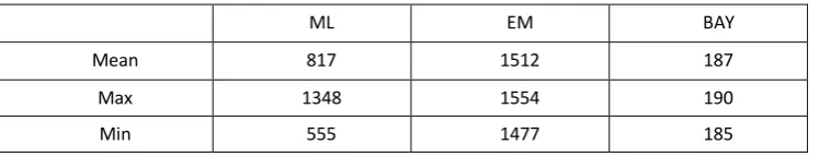
The last but not the least aspect of comparison is speed. Before the discussion, we reiterate that the speed have much to do with the quality of the codes, the software platform and the ability of the programmer. Best efforts have been made by the author to make the code run faster. As is seen from Table 3.1.5, the average computation time for each sample (of size 2000) is 187 seconds for Bayesian simulators, 817 seconds for ML and 1512 seconds for EM. The speed advantage of Bayesian approach is apparent for high dimensional SUR systems. Also note that the speed of Bayesian simulator is predictable and controllable since it is perfectly proportional to the number of draws. That is not the case in ML, because we have no exact idea how many iterations are needed to achieve convergence, nor how many function evaluations in the line search during the iteration.

We intentionally test the codes in Matlab since she has exceedingly good debugging tools and speed profiler. Latest version of Matlab has remarkable improvement in executing codes in the loop structure, and our coded in Fortran “.mex” files do not substantially increase the speed. Furthermore, we circumvent the slow Matlab optimization toolbox and use our own BFGS codes in ML estimation. Our test shows that the bottleneck of the ML is millions of the normal c.d.f. evaluation in the adapted GHK simulator, which accounts for about 80% of total CPU time. The bottle neck of EM algorithm turns out to be the truncated normal draws in the Monte-Carlo E step (50% of the CPU time). We used Geweke (1991)’s mixed source reject sampling to obtain the truncated normal and multivariate normal draws. The algorithm is indeed much faster than the inversion of normal c.d.f. But clearly millions or even billions of draws still requires substantial computation. Computation of Bayesian approach is light and CPU time is roughly evenly distributed in draws of truncated normal, Wishart matrix as well as inverted gamma draws. The only unfavorable aspect of Bayesian Gibbs sampler is that the memory usage is large. But nowadays RAMs are measured in GB and their I/O speed is several GBs per seconds. Therefore, high memory consumption becomes less relevant and matrix-oriented computation may accelerate the codes, especially ideal for the multi-core CPU.

Table 3.1.1 Censoring regime of generated data

number censored

censoring regime

2 (0,+,0,+) 4.07% 2 (0,+,+,0) 3.86% 2 (+,0,0,+) 3.24% 2 (+,0,+,0) 3.26% 2 (+,+,0,0) 3.08% 3 (0,0,0,+) 1.71% 3 (0,0,+,0) 1.61% 3 (0,+,0,0) 1.42% 3 (+,0,0,0) 1.12% 4 (0,0,0,0) 0.66%

Note:

“+” means non-censor,

“0” means censor to zero

Table 3.1.2 Inconsistency of OLS and GLS

TRUE OLS OLS_STD OLS_MSE GLS GLS_STD GLS_MSE

β11 1 1.345 0.022 0.120 1.345 0.022 0.120

β12 1 0.714 0.024 0.082 0.714 0.023 0.082

β13 1 0.707 0.022 0.086 0.708 0.022 0.086

β21 2 2.478 0.032 0.230 2.478 0.032 0.230

β22 2 1.488 0.029 0.263 1.487 0.028 0.264

β23 2 1.481 0.034 0.271 1.481 0.034 0.270

β31 3 3.652 0.033 0.426 3.652 0.033 0.426

β32 3 2.254 0.039 0.558 2.255 0.040 0.557

β33 3 2.250 0.039 0.565 2.250 0.039 0.565

β41 4 4.834 0.039 0.697 4.834 0.039 0.697

β42 4 3.017 0.052 0.969 3.018 0.052 0.968

β43 4 3.017 0.054 0.970 3.018 0.053 0.967

Σ11 1 0.980 0.047 0.003 0.980 0.047 0.003

Σ21 0.3 0.235 0.038 0.006 0.236 0.038 0.006

Σ31 0.3 0.237 0.038 0.005 0.237 0.038 0.005

Σ41 0.3 0.232 0.042 0.006 0.233 0.042 0.006

Σ22 1 1.441 0.062 0.198 1.441 0.062 0.198

Σ32 0.3 0.249 0.048 0.005 0.249 0.048 0.005

Σ42 0.3 0.248 0.052 0.005 0.248 0.052 0.005

Σ33 1 2.087 0.085 1.189 2.087 0.085 1.190

Σ43 0.3 0.255 0.070 0.007 0.256 0.070 0.007

Σ44 1 2.975 0.136 3.921 2.975 0.136 3.921

Note:

Table 3.1.3 comparison of ML, EM and Bayesian, individual estimators

ML EM

BAYESIA N

TRUE

MEA

N STD MSE

MEA

N STD MSE

MEA

N STD MSE

β11 1 1.000 0.034 0.001 1.006 0.047 0.002 1.001 0.030 0.001

β12 1 0.992 0.033 0.001 1.003 0.059 0.003 1.004 0.029 0.001

β13 1 0.987 0.029 0.001 0.999 0.055 0.003 0.998 0.026 0.001

β21 2 1.993 0.041 0.002 2.012 0.094 0.009 2.000 0.031 0.001

β22 2 1.997 0.030 0.001 1.993 0.107 0.011 2.002 0.027 0.001

β23 2 1.994 0.031 0.001 1.984 0.095 0.009 1.997 0.030 0.001

β31 3 2.993 0.032 0.001 2.985 0.145 0.021 2.999 0.029 0.001

β32 3 3.002 0.035 0.001 3.011 0.167 0.028 2.998 0.028 0.001

β33 3 3.000 0.033 0.001 3.005 0.191 0.036 2.996 0.027 0.001

β41 4 3.998 0.038 0.001 3.984 0.159 0.025 3.992 0.032 0.001

β42 4 4.018 0.041 0.002 3.993 0.267 0.071 4.003 0.032 0.001

β43 4 4.019 0.033 0.001 3.966 0.257 0.066 4.005 0.029 0.001

Σ11 1 0.949 0.051 0.005 1.016 0.048 0.003 0.989 0.041 0.002

Σ21 0.3 0.292 0.039 0.002 0.300 0.030 0.001 0.294 0.029 0.001

Σ31 0.3 0.301 0.031 0.001 0.303 0.028 0.001 0.295 0.026 0.001

Σ41 0.3 0.280 0.041 0.002 0.300 0.033 0.001 0.293 0.031 0.001

Σ22 1 0.959 0.056 0.005 1.031 0.046 0.003 0.994 0.043 0.002

Σ32 0.3 0.301 0.041 0.002 0.304 0.032 0.001 0.298 0.030 0.001

Σ42 0.3 0.273 0.040 0.002 0.301 0.038 0.001 0.296 0.029 0.001

Σ33 1 0.971 0.058 0.004 1.068 0.064 0.009 0.992 0.039 0.002

Σ43 0.3 0.232 0.064 0.009 0.303 0.043 0.002 0.297 0.032 0.001

Σ44 1 0.974 0.064 0.005 1.113 0.130 0.030 0.990 0.041 0.002

DF 6 5.552 0.516 0.464 6.428 0.537 0.469 6.016 0.491 0.239

Note:

Estimators (ML,EM,BAY) are the sample mean of estimators of 100 experiments. Standard errors are the sample standard deviations, MSEs are also sample analog.

Table 3.1.4 comparison of ML, EM and Bayesian, composite estimators

ML EM BAY

Quadric risk of β 0.015 0.285 0.010

MSE definiteness MSE(ML β) – MSE(EM β) < 0 , others not comparable

Table 3.1.5 computation time of ML, EM and Bayesian approach (Seconds)

ML EM BAY

Mean 817 1512 187

Max 1348 1554 190

Min 555 1477 185

Note: computation time is ONE experiment with 2000 observations Intel Pentium Dual 2.5GHZ / 3GB RAM / 64 bit Vista / Matlab 2009a

3.2 Effects of sample size

As we know, if the data generating process is exactly the same as what is described in Section 3.1, then the ML, EM and BAY estimators should get closer and closer to the true parameters as the sample size goes to infinity. In practice, however, every data set is of finite size. Now we conduct a series of experiments with varied sample size, and our goal is to answer the question “How large is large?” for each estimation method.

The sample sizes are set to be respectively.

One limitation of this study is that it takes hours to estimate the model with 20000 observations. Therefore, it is infeasible to conduct repeated experiments for hundreds of times (on my computer). Since we only do it once, the estimators might be less stable due to sampling randomness. The statistics should be read with reference to asymptotical standard errors.

The major findings of those experiments are Bayesian approach performs satisfactorily even under relatively small sample and computation speed increases moderately as sample size grows, compared with ML and EM estimators.

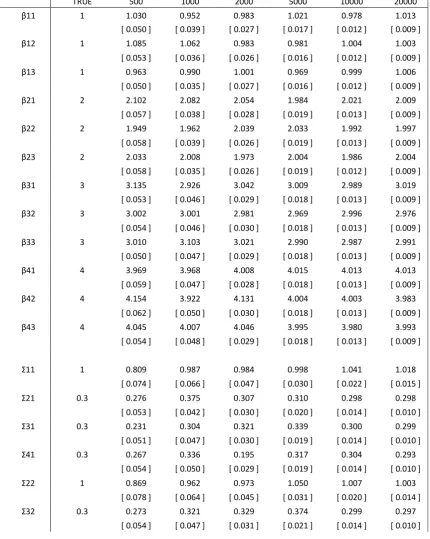
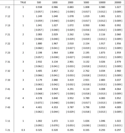
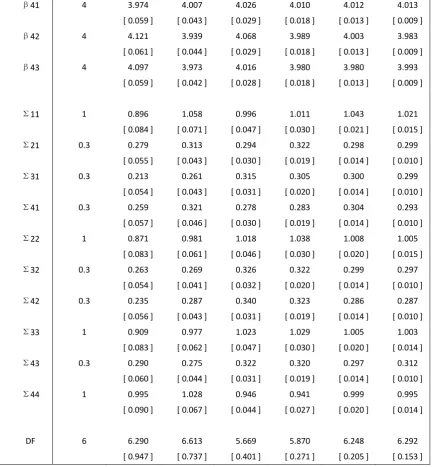
As is seen in Table 3.2.1 – 3.2.4, in the case of , ML and EM estimators exhibit apparent deviation from the true coefficients. Particularly, the degree of freedom parameter wanders far from

. However, Bayesian estimator works much better—regression coefficients, covariance matrix and degree of freedom estimators are all reasonably close to the true parameters. The quadratic risks (the squared sum of estimator deviations) are 0.026 for ML, 0.131 for EM and merely 0.009 for Bayesian estimators.

To attain the same quality, the costs are of great disparity. To estimate the data set of 20000, it takes roughly 5.3 hours via ML, 4.5 hours via EM, but merely 45 minutes by Bayesian approach. The savings of Bayesian estimators are awesome. Furthermore, the speed of Gibbs sampler is almost perfectly predictable, so that the researcher can add a status bar when the codes are running, watching and planning ahead. However, for ML estimator, the researcher never knows how many iterations it will take, so he waits and wishes it could end sooner.

Table 3.2.1 ML estimators with varied sample size

TRUE 500 1000 2000 5000 10000 20000

β11 1 1.030 0.952 0.983 1.021 0.978 1.013 [ 0.050 ] [ 0.039 ] [ 0.027 ] [ 0.017 ] [ 0.012 ] [ 0.009 ]

β12 1 1.085 1.062 0.983 0.981 1.004 1.003 [ 0.053 ] [ 0.036 ] [ 0.026 ] [ 0.016 ] [ 0.012 ] [ 0.009 ]

β13 1 0.963 0.990 1.001 0.969 0.999 1.006 [ 0.050 ] [ 0.035 ] [ 0.027 ] [ 0.016 ] [ 0.012 ] [ 0.009 ]

β21 2 2.102 2.082 2.054 1.984 2.021 2.009 [ 0.057 ] [ 0.038 ] [ 0.028 ] [ 0.019 ] [ 0.013 ] [ 0.009 ]

β22 2 1.949 1.962 2.039 2.033 1.992 1.997 [ 0.058 ] [ 0.039 ] [ 0.026 ] [ 0.019 ] [ 0.013 ] [ 0.009 ]

β23 2 2.033 2.008 1.973 2.004 1.986 2.004 [ 0.058 ] [ 0.035 ] [ 0.026 ] [ 0.019 ] [ 0.012 ] [ 0.009 ]

β31 3 3.135 2.926 3.042 3.009 2.989 3.019 [ 0.053 ] [ 0.046 ] [ 0.029 ] [ 0.018 ] [ 0.013 ] [ 0.009 ]

β32 3 3.002 3.001 2.981 2.969 2.996 2.976 [ 0.054 ] [ 0.046 ] [ 0.030 ] [ 0.018 ] [ 0.013 ] [ 0.009 ]

β33 3 3.010 3.103 3.021 2.990 2.987 2.991 [ 0.050 ] [ 0.047 ] [ 0.029 ] [ 0.018 ] [ 0.013 ] [ 0.009 ]

β41 4 3.969 3.968 4.008 4.015 4.013 4.013 [ 0.059 ] [ 0.047 ] [ 0.028 ] [ 0.018 ] [ 0.013 ] [ 0.009 ]

β42 4 4.154 3.922 4.131 4.004 4.003 3.983 [ 0.062 ] [ 0.050 ] [ 0.030 ] [ 0.018 ] [ 0.013 ] [ 0.009 ]

β43 4 4.045 4.007 4.046 3.995 3.980 3.993 [ 0.054 ] [ 0.048 ] [ 0.029 ] [ 0.018 ] [ 0.013 ] [ 0.009 ]

Σ11 1 0.809 0.987 0.984 0.998 1.041 1.018 [ 0.074 ] [ 0.066 ] [ 0.047 ] [ 0.030 ] [ 0.022 ] [ 0.015 ]

Σ21 0.3 0.276 0.375 0.307 0.310 0.298 0.298 [ 0.053 ] [ 0.042 ] [ 0.030 ] [ 0.020 ] [ 0.014 ] [ 0.010 ]

Σ31 0.3 0.231 0.304 0.321 0.339 0.300 0.299 [ 0.051 ] [ 0.047 ] [ 0.030 ] [ 0.019 ] [ 0.014 ] [ 0.010 ]

Σ41 0.3 0.267 0.336 0.195 0.317 0.304 0.293 [ 0.054 ] [ 0.050 ] [ 0.029 ] [ 0.019 ] [ 0.014 ] [ 0.010 ]

Σ22 1 0.869 0.962 0.973 1.050 1.007 1.003 [ 0.078 ] [ 0.064 ] [ 0.045 ] [ 0.031 ] [ 0.020 ] [ 0.014 ]

Σ42 0.3 0.171 0.269 0.296 0.308 0.286 0.286 [ 0.055 ] [ 0.048 ] [ 0.028 ] [ 0.020 ] [ 0.014 ] [ 0.010 ]

Σ33 1 0.849 1.113 0.989 1.018 1.004 1.001 [ 0.080 ] [ 0.082 ] [ 0.045 ] [ 0.030 ] [ 0.020 ] [ 0.014 ]

Σ43 0.3 0.280 0.147 0.227 0.288 0.296 0.311 [ 0.057 ] [ 0.055 ] [ 0.029 ] [ 0.019 ] [ 0.014 ] [ 0.010 ]

Σ44 1 0.980 1.172 0.874 0.912 0.998 0.993 [ 0.094 ] [ 0.084 ] [ 0.040 ] [ 0.027 ] [ 0.020 ] [ 0.014 ]

DF 6 5.346 5.323 5.265 5.254 6.194 6.215 [ 0.807 ] [ 0.638 ] [ 0.382 ] [ 0.243 ] [ 0.210 ] [ 0.148 ]

Note: (Asymptotical) Standard errors are reported in brackets.

Table 3.2.2 EM estimators with varied sample size

TRUE 500 1000 2000 5000 10000 20000

β11 1 0.938 0.986 0.883 1.008 0.980 1.027 [ 0.057 ] [ 0.041 ] [ 0.030 ] [ 0.017 ] [ 0.012 ] [ 0.009 ]

β12 1 1.249 1.040 1.078 1.019 1.001 1.021 [ 0.059 ] [ 0.040 ] [ 0.029 ] [ 0.017 ] [ 0.012 ] [ 0.009 ]

β13 1 1.041 1.027 1.072 0.950 0.965 0.992 [ 0.057 ] [ 0.040 ] [ 0.029 ] [ 0.016 ] [ 0.012 ] [ 0.009 ]

β21 2 2.083 2.029 2.262 1.916 2.116 2.060 [ 0.060 ] [ 0.040 ] [ 0.029 ] [ 0.019 ] [ 0.012 ] [ 0.009 ]

β22 2 1.880 1.967 2.010 2.154 1.917 1.956 [ 0.060 ] [ 0.041 ] [ 0.027 ] [ 0.019 ] [ 0.012 ] [ 0.009 ]

β23 2 2.198 1.964 1.858 2.195 1.873 1.959 [ 0.057 ] [ 0.038 ] [ 0.027 ] [ 0.020 ] [ 0.012 ] [ 0.009 ]

β31 3 2.932 3.134 2.901 3.132 3.026 2.979 [ 0.062 ] [ 0.041 ] [ 0.033 ] [ 0.018 ] [ 0.013 ] [ 0.009 ]

β32 3 3.405 2.857 3.152 2.762 3.034 2.960 [ 0.066 ] [ 0.041 ] [ 0.033 ] [ 0.018 ] [ 0.013 ] [ 0.009 ]

β33 3 3.179 2.880 3.419 2.921 2.883 3.037 [ 0.063 ] [ 0.042 ] [ 0.032 ] [ 0.018 ] [ 0.013 ] [ 0.009 ]

β41 4 3.648 3.918 4.291 4.114 4.008 4.064 [ 0.068 ] [ 0.047 ] [ 0.030 ] [ 0.018 ] [ 0.013 ] [ 0.009 ]

β42 4 4.578 3.840 3.952 3.789 4.083 3.952 [ 0.072 ] [ 0.048 ] [ 0.030 ] [ 0.017 ] [ 0.013 ] [ 0.009 ]

β43 4 4.401 4.353 3.787 3.798 3.959 4.009 [ 0.062 ] [ 0.044 ] [ 0.029 ] [ 0.018 ] [ 0.013 ] [ 0.009 ]

Σ11 1 1.002 1.072 1.113 1.026 1.046 1.022 [ 0.092 ] [ 0.070 ] [ 0.053 ] [ 0.030 ] [ 0.022 ] [ 0.015 ]

[ 0.062 ] [ 0.043 ] [ 0.033 ] [ 0.020 ] [ 0.013 ] [ 0.009 ]

Σ31 0.3 0.257 0.259 0.340 0.305 0.299 0.301 [ 0.068 ] [ 0.043 ] [ 0.035 ] [ 0.019 ] [ 0.014 ] [ 0.010 ]

Σ41 0.3 0.304 0.335 0.273 0.281 0.305 0.293 [ 0.066 ] [ 0.050 ] [ 0.034 ] [ 0.019 ] [ 0.014 ] [ 0.010 ]

Σ22 1 0.987 1.016 1.047 1.117 0.994 0.995 [ 0.083 ] [ 0.065 ] [ 0.047 ] [ 0.033 ] [ 0.020 ] [ 0.014 ]

Σ32 0.3 0.275 0.258 0.325 0.324 0.293 0.295 [ 0.064 ] [ 0.042 ] [ 0.035 ] [ 0.021 ] [ 0.014 ] [ 0.010 ]

Σ42 0.3 0.256 0.318 0.361 0.330 0.282 0.286 [ 0.067 ] [ 0.047 ] [ 0.031 ] [ 0.020 ] [ 0.014 ] [ 0.010 ]

Σ33 1 1.142 0.991 1.210 1.037 1.014 1.016 [ 0.113 ] [ 0.065 ] [ 0.056 ] [ 0.030 ] [ 0.020 ] [ 0.015 ]

Σ43 0.3 0.387 0.296 0.333 0.313 0.297 0.312 [ 0.078 ] [ 0.049 ] [ 0.035 ] [ 0.019 ] [ 0.014 ] [ 0.010 ]

Σ44 1 1.292 1.209 0.999 0.961 1.015 0.994 [ 0.129 ] [ 0.082 ] [ 0.045 ] [ 0.028 ] [ 0.020 ] [ 0.014 ]

DF 6 7.396 6.898 6.188 6.050 6.327 6.297 [ 1.283 ] [ 0.795 ] [ 0.477 ] [ 0.281 ] [ 0.216 ] [ 0.150 ]

Note: (Asymptotical) Standard errors are reported in brackets.

Table 3.2.3 Bayesian estimators with varied sample size

TRUE 500 1000 2000 5000 10000 20000

β11 1 1.015 0.957 1.001 1.015 0.977 1.012 [ 0.052 ] [ 0.040 ] [ 0.028 ] [ 0.017 ] [ 0.012 ] [ 0.009 ]

β12 1 1.098 1.053 0.982 0.998 1.004 1.004 [ 0.053 ] [ 0.039 ] [ 0.026 ] [ 0.017 ] [ 0.012 ] [ 0.009 ]

β13 1 0.979 1.018 1.008 0.989 0.999 1.006 [ 0.052 ] [ 0.039 ] [ 0.027 ] [ 0.016 ] [ 0.012 ] [ 0.009 ]

β21 2 2.129 2.085 2.048 1.992 2.021 2.008 [ 0.052 ] [ 0.039 ] [ 0.029 ] [ 0.018 ] [ 0.013 ] [ 0.009 ]

β22 2 1.926 1.960 2.023 2.040 1.992 1.997 [ 0.055 ] [ 0.038 ] [ 0.028 ] [ 0.018 ] [ 0.013 ] [ 0.009 ]

β23 2 2.013 1.969 1.969 2.008 1.986 2.004 [ 0.052 ] [ 0.038 ] [ 0.028 ] [ 0.018 ] [ 0.013 ] [ 0.009 ]

β31 3 3.113 2.923 3.057 3.020 2.989 3.018 [ 0.056 ] [ 0.042 ] [ 0.029 ] [ 0.018 ] [ 0.013 ] [ 0.009 ]

β32 3 3.019 2.965 3.003 2.961 2.996 2.976 [ 0.057 ] [ 0.040 ] [ 0.030 ] [ 0.018 ] [ 0.013 ] [ 0.009 ]

β41 4 3.974 4.007 4.026 4.010 4.012 4.013 [ 0.059 ] [ 0.043 ] [ 0.029 ] [ 0.018 ] [ 0.013 ] [ 0.009 ]

β42 4 4.121 3.939 4.068 3.989 4.003 3.983 [ 0.061 ] [ 0.044 ] [ 0.029 ] [ 0.018 ] [ 0.013 ] [ 0.009 ]

β43 4 4.097 3.973 4.016 3.980 3.980 3.993 [ 0.059 ] [ 0.042 ] [ 0.028 ] [ 0.018 ] [ 0.013 ] [ 0.009 ]

Σ11 1 0.896 1.058 0.996 1.011 1.043 1.021 [ 0.084 ] [ 0.071 ] [ 0.047 ] [ 0.030 ] [ 0.021 ] [ 0.015 ]

Σ21 0.3 0.279 0.313 0.294 0.322 0.298 0.299 [ 0.055 ] [ 0.043 ] [ 0.030 ] [ 0.019 ] [ 0.014 ] [ 0.010 ]

Σ31 0.3 0.213 0.261 0.315 0.305 0.300 0.299 [ 0.054 ] [ 0.043 ] [ 0.031 ] [ 0.020 ] [ 0.014 ] [ 0.010 ]

Σ41 0.3 0.259 0.321 0.278 0.283 0.304 0.293 [ 0.057 ] [ 0.046 ] [ 0.030 ] [ 0.019 ] [ 0.014 ] [ 0.010 ]

Σ22 1 0.871 0.981 1.018 1.038 1.008 1.005 [ 0.083 ] [ 0.061 ] [ 0.046 ] [ 0.030 ] [ 0.020 ] [ 0.015 ]

Σ32 0.3 0.263 0.269 0.326 0.322 0.299 0.297 [ 0.054 ] [ 0.041 ] [ 0.032 ] [ 0.020 ] [ 0.014 ] [ 0.010 ]

Σ42 0.3 0.235 0.287 0.340 0.323 0.286 0.287 [ 0.056 ] [ 0.043 ] [ 0.031 ] [ 0.019 ] [ 0.014 ] [ 0.010 ]

Σ33 1 0.909 0.977 1.023 1.029 1.005 1.003 [ 0.083 ] [ 0.062 ] [ 0.047 ] [ 0.030 ] [ 0.020 ] [ 0.014 ]

Σ43 0.3 0.290 0.275 0.322 0.320 0.297 0.312 [ 0.060 ] [ 0.044 ] [ 0.031 ] [ 0.019 ] [ 0.014 ] [ 0.010 ]

Σ44 1 0.995 1.028 0.946 0.941 0.999 0.995 [ 0.090 ] [ 0.067 ] [ 0.044 ] [ 0.027 ] [ 0.020 ] [ 0.014 ]

DF 6 6.290 6.613 5.669 5.870 6.248 6.292 [ 0.947 ] [ 0.737 ] [ 0.401 ] [ 0.271 ] [ 0.205 ] [ 0.153 ]

Note: (Asymptotical) Standard errors are reported in brackets.

Table 3.2.4 Comparison of quadratic risk

500 1000 2000 5000 10000 20000 ML 0.026 0.025 0.026 0.025 0.002 0.002 EM 0.131 0.047 0.024 0.012 0.007 0.005 BAY 0.009 0.018 0.006 0.001 0.003 0.004

500 1000 2000 5000 10000 20000 ML 173 556 873 2243 9412 19176 EM 635 967 1600 3811 7905 16153 BAY 66 105 192 540 1122 2660

4. Application

4.1 The topic

In this section, we apply the SUR Tobit scale-mixture model to high frequency financial data, and will study the interaction between security price and trading volume.

In finance, there is dichotomy between the academia and the practitioners on technical analysis. Chartists forecast future stock price using various figures patterns, formulas and indicators, the inputs of which are essentially two: historical prices and trading volumes. One of the popular indicators is moving average (MA) crossings (i.e. filtering rules). When, for example, the short-run MA line cuts the long-run MA line from the bottom, it is a buying signal. In a highly simplified model, we will show the above filtering-rule trading strategy could admit a Vector Auto-Regression (VAR) representation consisting of price and volume.

However, the informational value of past prices and trading volumes is underappreciated in academia in general. Many of us are happy with the Efficient Market Hypothesis (Fama, 1965). The argument is that there is no free lunch in Wall Street since the current price has already contains all the historical information; technical analysis, therefore, is in vain. The implication for the econometric model is that the lagged regressors will have no explanatory power on the current price.

Time series analysis to the technical analysis, is something like astronomy to the astrology. Campbell et al. (1997) insightfully pointed out that despite the linguistic barriers, time series and technical analysis do study the same thing—the informational content of historical prices. Studies by Brock et al. (1992), Taylor and Allen (1992), Lo et.al (2000) provided some foundations of technical analysis from the perspective of statistics.

Basically what we do in this section is to run a VAR model, study the associated impulse response functions and test the significance of lagged explanatory variables. As we are taught in the textbook,

“Vector auto-regressions are invariably estimated on the basis of conditional likelihood function rather than the full sample unconditional likelihood.” (Hamilton, 1994). The conditional ML turns out to be OLS equation by equation. However, when the model is applied to high frequency data recorded in seconds intervals, there are at least two complications:

1. There might be no transactions in a certain time interval, hence zero trading volume. 2. High frequency data are well-known to exhibit non-normality, typically with a fatter tail.

The first issue can be viewed as censored observation around zero. Since the censored data could constitute a non-negligible portion, the OLS will be apparently inconsistent.

Even if in the absence of the first issue, the presence of the second issue may render the OLS less efficient. The fat tail can be largely addressed by models with scale-mixture errors.

correction, etc). Since we are dealing with very high frequency data, it stands to reason to believe shocks within a minute come from idiosyncratic sources such as individuals or institutional investors. The micro-sourced shocks should not have impacts last forever. Therefore there is no good reason to worry about the unit root, let alone the cointegrating constraints. With this assumption, we can simply treat the reduced form VAR as a SUR model, and denote all the predetermined lagged variables , and all the coefficients , so that we can use all the micro-econometric methods to estimate the model.

All in all, the model we use is essentially the SUR Tobit system with scale-mixture errors, exactly as is described in Section 2.1

4.2 The simple model

To justify the use of VAR, we provide a highly simplified (maybe trivial) model of investors’ behavior and determination of price and volumes.

The investors are assumed to be chartists who use filtering rule on the basis of MA lines to determine the quote and the amount to buy/sell. Since actual transactions do occur, agents must be heterogeneous (If agents’ preference are identical, price could be pinned down when the market clears, but no transaction indeed. Another possibility is to introduce other type of investors such as risk-averse hedgers, fundamentalists, noise traders, etc. That leaves for future research. )

Let the historical price be { }

, the moving average chart of order q can be written as:

∑

In a call auction mechanism, an investor places her limit orders with desired price and quantity, which, by assumption, is determined by the differences of various MA lines. In its reduced form, this is equivalent to be determined by weighted average of MA lines.

If she is a potential buyer,

Desired buying price: ∑ Desired amount: ∑ ̃ If she is a potential seller,

Desired selling price: ∑ Desired amount: ∑ ̃

Where the weights , ̃ reflects the individual’s preference and judgment.

The price that enables the largest number of orders to be executed is then chosen. The market clearing requires:

∑ ( ) ∑ ( )

The trading volume ∑ ( )

Where ( ) is the indicator function that takes the value of 1 if the expression in bracket are true, and 0 otherwise.

Apparently, both the and are linear functions of moving average lines, hence linear with respect to historical prices and trading volumes.

In econometrics, this implies a VAR representation of price and volumes

Where ( *

The disturbance could be interpreted as the change of individual’s taste, measure errors, etc.

4.3 Data and estimation

Issued in August 22, 2005, Baosteel warrants (a type of call options) was the first financial derivatives traded in Shanghai Stock Exchange, China. The options were spectacular in that its price featured extreme volatility and 5-10 times higher than what Black-Scholes formula implied. Academia, in general, could not provide convincing rationales why the options price wandered far away from the fundamentals—bubbles, they guess. It is believed that the participants are all speculative individuals who may sell the options minutes after purchase. At that time, maybe only the chartists took delight in talking about its price movement and trading strategies.

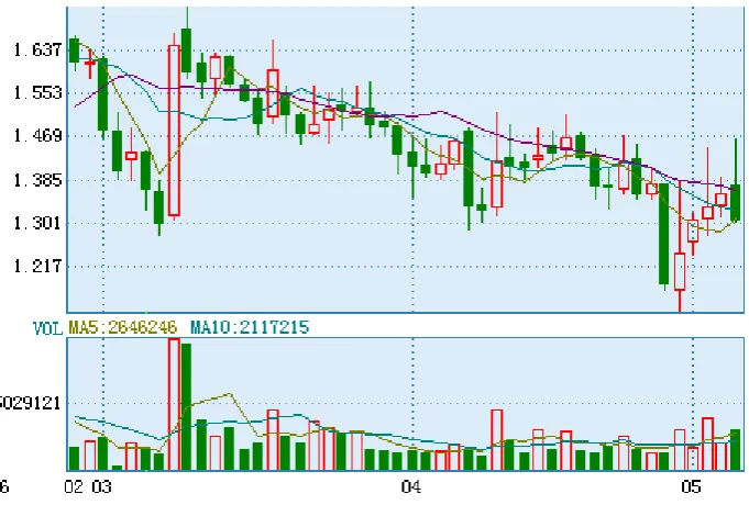
We use price and volume data of 30 consecutive trading days starting from March 23, 2006. Each day has four trading hours. The frequency of the data is 3 seconds. So we have the sample size of 144,000. In this high frequency data set, 21.94% of the volume data are recorded as zero, implying no transaction in that time interval.

Figure 4.3.1 Price sequence (candlesticks) and trading volume

Note: As the convention, candlestick chart are based on daily trading data.

To run a VAR regression, we need to choose a proper lag length, which can be determined by the Schwarz information criterion (SIC):

Where is the log-likelihood function, k is number of regressors and T is number of observations. Apparently, to perform SIC, one must run the regression for every lag specification, say, from 1 lag model to 100 lags model. That is too much computation for our model with censoring and scale-mixtures. So when we choose the lag structure, we neglect the two complications and use the equation-wise-OLS based conditional likelihood. This is not very correct, strictly speaking, but merely some expediency. The SIC suggests lag length of 27.

When we estimate the VAR with 27 lags, we do use the full information maximum likelihood and Bayesian approach, as is described in Section 2.1. Since the Monte Carlo experiments in Section 3 suggest poor performance of the slow EM algorithm, we do not use that approach here.

In this application, the model is a bivariate SUR Tobit. It is important to note that numerical algorithms are different for lower and higher dimensional problems. For instance, in lower dimension, Gaussian quadratures usually provides a much faster and more accurate approximation, while Monte Carlo methods are more suitable for higher dimensional problem because it suffers less from the curse of dimension.

For speed and accuracy, in this bivariate system, Gaussian quadratures are employed instead of direct Monte Carlo simulation whenever possible. In maximum likelihood, the probability of censored observation is essentially an integrand consisting of a univarite normal c.d.f. and an IG p.d.f.. If we took thousands of IG draws to directly simulate the probability, it would be too slow. We instead divide the integration range into subintervals and use Gauss-Laguerre and Gauss-Legendre quadratures accordingly. In that fashion, hundreds of weighed sum of univarite normal c.d.f. will provide a much faster and more accurate censoring probability.

Another feature of VAR model is the presence of a large amount of regressors. With 27 lags, there are 108 lagged explanatory variables (and 2 constants), plus covariance matrix and degree of freedom parameters. To accelerate the codes, it is also important to provide the analytic gradient in ML estimation. If we let the computer to calculate the numerical derivatives, it would require excessive calls to the objective function. Analytic gradients, however, requires little additional computer’s efforts (but substantial human debugging efforts!), so that the codes could be ten times faster.

Estimation results are provided in Table 4.3.1. The left column is ML estimators and the right column is Bayesian simulators (posterior mean). Since large amount of regressors consume so much paper space, the standard errors are not reported for ecological reasons. (They are available upon request.) In fact, the covariance matrix of estimators is useful in that later we need it to calculate 95% intervals of impulse response functions. As we can see from the table, the ML and Bayesian approach produce very similar results. The coefficients corresponding to the first lag are relatively large, and decay with the lags. The estimated degree of freedom is very small, implying that the disturbance terms do deviate from normality to a large extend.

the interval since we already have posterior draws. For each draw, we invert the VAR into ( ) representation and the coefficients are response magnitudes. Repeat for all draws, the 2.5% and 97.5% percentiles are the two boundaries of the 95% intervals. As for the ML approach, we assume the normality of estimators (though the disturbances are scale mixtures, the ML estimators should be asymptotically normal anyway), so that we can use parametric bootstrap to obtain simulated draws of estimators, get

( ) representations and depict the 95% intervals.

Finally, we test the information contents of historical price and trading volumes. The easiest way to test the null (namely efficient market hypothesis) is LR test which has distribution asymptotically. Simply remove all the lagged regressors, as we expect, the log likelihood decreases drastically, thus the efficient market hypothesis is rejected in our model.

Table 4.3.1 Reduced form VAR estimation

ML BAY

Eq(1) Eq(2) Eq(1) Eq(2) Const 0.003 -0.007 0.003 -0.006

ф(1) 0.894 0.003 0.887 0.003 0.000 0.044 -0.001 0.054

ф(2) -0.005 0.005 -0.002 0.005 0.001 0.034 0.000 0.035

ф(3) 0.041 0.001 0.042 0.000 0.002 0.028 0.001 0.028

ф(4) 0.024 0.003 0.025 0.003 -0.002 0.028 -0.002 0.028

ф(5) 0.013 -0.001 0.014 -0.001 -0.001 0.023 -0.001 0.023

ф(6) 0.023 0.000 0.024 -0.001 0.000 0.022 0.000 0.022

ф(7) 0.020 0.001 0.020 0.001 -0.001 0.016 -0.001 0.016

ф(8) 0.017 0.003 0.017 0.003 0.001 0.019 0.001 0.019

ф(9) 0.015 0.000 0.016 0.000 0.003 0.017 0.004 0.017

ф(10) 0.010 -0.001 0.010 -0.001 0.000 0.019 0.000 0.020

ф(11) 0.000 -0.001 0.000 -0.001 0.002 0.019 0.002 0.019

ф(12) -0.001 -0.003 -0.002 -0.003 0.004 0.015 0.003 0.015

ф(13) 0.000 0.000 0.000 0.000 0.000 0.017 0.001 0.017

0.001 0.017 0.001 0.018

ф(15) -0.008 -0.001 -0.009 -0.001 0.001 0.017 0.001 0.017

ф(16) -0.005 -0.001 -0.005 -0.001 -0.003 0.012 -0.004 0.012

ф(17) -0.004 -0.001 -0.004 -0.001 0.000 0.015 0.001 0.015

ф(18) -0.007 -0.002 -0.007 -0.002 -0.002 0.016 -0.003 0.016

ф(19) -0.005 -0.001 -0.005 -0.001 0.000 0.014 0.000 0.014

ф(20) -0.002 -0.001 -0.002 -0.001 0.001 0.015 0.000 0.015

ф(21) -0.001 -0.001 -0.001 -0.001 -0.003 0.014 -0.002 0.014

ф(22) -0.002 0.000 -0.002 0.000 -0.003 0.011 -0.002 0.012

ф(23) -0.003 -0.003 -0.003 -0.003 0.001 0.013 0.001 0.014

ф(24) -0.003 -0.001 -0.003 -0.001 -0.003 0.015 -0.003 0.015

ф(25) -0.002 0.001 -0.002 0.001 -0.003 0.013 -0.003 0.013

ф(26) 0.001 0.001 0.001 0.001 0.004 0.012 0.004 0.012

ф(27) -0.001 -0.001 -0.001 -0.001 0.000 0.013 0.001 0.014

Σ 1.52E-03 -2.28E-05 1.45E-03 -2.24E-05 -2.28E-05 1.91E-03 -2.24E-05 1.91E-03 DF 1.469 1.409

Note:

The left panel is the response of price to the price shocks. The right panel is the response of volume to the price shocks.

Figure 4.3.3 Response to price shocks, Bayesian estimation

Note:

The left panel is the response of price to the price shocks. The right panel is the response of volume to the price shocks.

Figure 4.3.4 Response to volume shocks, ML estimation

0 10 20 30 40 50

0.025 0.03 0.035 0.04 0.045

Price Response

0 20 40 60 80

-2 0 2 4 6x 10

-4

Volume Response

0 10 20 30 40 50

0.025 0.03 0.035 0.04 0.045

Price Response

0 20 40 60 80

-4 -2 0 2 4 6x 10

-4

Note:

The left panel is the response of price to the volume shocks. The right panel is the response of volume to the volume shocks.

Figure 4.3.5 Response to volume shocks, Bayesian estimation

Note:

The left panel is the response of price to the volume shocks. The right panel is the response of volume to the volume shocks.

5. Extensions

In this section, we extend the scale-mixture SUR Tobit model in two directions. Firstly, we keep the scale-mixture assumption and extend the model to incidental truncation, namely sample selection models. Secondly, we keep the basic Tobit specification, but extend the disturbance terms to finite Gaussian regime mixtures, which in principle can imitate any shape of distribution.

0 20 40 60 80 100

-2 -1 0 1x 10

-3

Price Response

0 5 10 15 20

0 0.01 0.02 0.03 0.04 0.05

Volume Response

0 20 40 60 80 100

-15 -10 -5 0 5x 10

-4 _{Price Response}

0 5 10 15 20

0 0.01 0.02 0.03 0.04 0.05

5.1 Sample selection model

In the benchmark model in Section 2.1, the censoring mechanism and activity levels are governed by the same stochastic process, that is, the variable is censored to zero whenever its value falls below zero. However, sometimes it is of interest to consider the separation of participation equation and the activity level equation. In other words, one variable could be incidentally censored whenever another related variable falls below zero.

The sample selection SUR Tobit with scale mixtures can be written as:

 Participation equations:

……

 Activity level equations:

……

 Selection mechanism:

( )

 Error specification:

( ) | ( ) , where is positive definite matrix . /

The and are observable, while the latent , , are not.

Essentially, the censoring rules are: will be censored to zero whenever falls below zero. In most applications, is an artifact constructed from the knowledge whether the observable is zero or not.

For future reference, stack the variables in the obvious way,

(

+ , (

+ , (

+ , (

+ ,

(

+ , (

+ , (

+ , (

+

( ) , ( )

( + , ( + , ( + , ( + , ( + , ( + , ( +

To discuss the estimation, we need some further notations.

Without loss of generality, for some individual t, rearrange the order of variables so that the first elements of are intact but the last variates are censored to zero. We use the

variables are partitioned to be: ( * , ( * , ( * , ( * , ( * , ( *, . / , ( * , . / , . / ( , ( , ̃

̃ is some permutation of conformable to the above variable rearrangement. The log likelihood is ∑ ( ) , where

( ) ∫ ∫ ∫ ( )

∫ ∫ ( )

( ) ∫ ∫ ( | )

( ) ∫ ∫ ∫ ( | ) ( | )

As a notation, variables and intervals have the order like ∫ ∫ ∫ ( )

It can be shown that

( )

| { 0 ( ) ( )1

}

| ( ̅ ̅)

Where ̅ (

* ( * ₍ ) ̅ [( * ( * _{( )]}

Obviously, simulation techniques must be used to evaluate the likelihood function. GHK simulator adapted for MVT c.d.f., as is described in Section 2.2, can be used to evaluate the integral.

Alternatively, the above sample selection model can also be estimated via EM or Bayesian approach. We briefly outline the steps as follows.

E-M algorithm:

The complete data log likelihood can be written as

( | ) ∑ , ( | ) ( | )- ∑ [ . / . / . / | | ₍ * ( * ]

We use the informal notation “constant” to represent those additive terms which do not interact with

The joint posterior distribution of does not have a recognizable form, but the conditional distribution does. | ( )( ̅ ̅ ) | ( )( ̅ ̅ ) | ( ̅ ̅ )

| { 6 ( _{* (} *7 } where ̅ ( ) ( + : ; ̅ ( ) ( + : ; ̅ ( ) ( + : ;

̅ < ( ) (

+ ( +=

̅ < ( ) ( + ( +=

̅ < ( ) (

+ ( +=

Make sure that are evaluated at estimators of last iteration.

With the posterior conditionals, Gibbs Sampler can be used to obtain draws:

{ ( ) ( ) ( ) ( ) ( )} , or more compactly { ( ) ( ) ( )} , .

The expected complete data likelihood then can be approximated by the ergodic mean:

, ( | )-

∑ ∑

[

. / . / . / ( ) ( )

( ) | | ( ) 4 ( )

( ) 5

₄ ( ) ( ) 5 ]

The conditional M-steps have the following cycling update rule of estimators:

. _{/ [∑} . ∑ _{( )} / ( * ฀ ฀ _{( *} ]

∑ 6( * 4 ∑ _{( )} 4 ( )

( )5 57