Long term interest rates, asset prices, and personal saving ratio: Evidence from the 1990s

Munich Personal RePEc Archive

Long-term interest rates, asset prices,

and personal saving ratio: Evidence from

the 1990s

Antonio, Paradiso

6 October 2010

Online at

https://mpra.ub.uni-muenchen.de/26754/

Long-term interest rates, asset prices, and personal saving ratio: Evidence from the

1990s

Antonio Paradisoa,

a

ISAE (Institute for Studies and Economic Analysis) and University of Rome La Sapienza

This article investigates the personal saving ratio in the US economy in the last two decades. We

examine whether the mortgage equity withdrawal (MEW) mechanism – the cash out from refinancing

home mortgage conditions – is useful for explaining the saving ratio’s declining pattern. Empirically, we

find that MEW depends on house price inflation and mortgage rates. We construct a VEC model among the two variables explaining MEW, the saving ratio and the stock price. We obtain a significant cointegrating relationship. We then estimate a structural form imposing restrictions, suggested by theoretical or empirical literature, on the long-run impact matrix. We find a negative response of the saving ratio to positive shocks in asset prices, whereas there is an opposite effect in the case of a positive shock in mortgage rates, according to the theoretical expectations.

Keywords: Saving ratio, MEW, VEC, asset prices, long-term interest rates

I Introduction

The huge decline in the personal saving rate in the US economy during the last two decades has raised interest among economists in identifying an explanation. Different theories/explanations have been put forth (see Guidolin and La Jeunesse 2007 for a review). A theory advanced mainly by practitioners and investors (Hatzius 2006) considers the mechanism of mortgage equity withdrawal (MEW) – equity extracted from existing houses via cash-out refinancing – as the main cause of the declining saving pattern. MEW acts as an additional channel beyond the traditional wealth effect through which increases in house prices can boost consumer spending. We show that the MEW income ratio depends mainly on the change in house prices (positively) and mortgage rate (negatively). This means that lower house prices might put upward pressure on the saving rate, whereas a reduction in mortgage rates might imply an opposite effect. In the logic of the MEW mechanism, house price inflation could have effects that are similar to those of an extra income to consumers.

To obtain direct evidence of the role of MEW in explaining the personal saving rate dynamic for the last two decades, we use directly the variables explaining the MEW – together with the stock price index – to estimate a VEC model. Our results confirm the presence of a significant long-run relationship among the saving ratio, stock price index, house price inflation, and mortgage rates. In our model, we identify the shocks with long-run restrictions in our empirical VEC. All the restrictions used are justifiable by theoretical or empirical models presented in the literature. The impulse response function (IRF) points out that the saving ratio reacts negatively to asset price shocks and positively to mortgage rate shocks, in a way consistent with our theoretical expectations.

II The empirical VEC model

The data

The variables used in the empirical VEC analysis are the house price index inflation (expressed in the year-on-year growth rate) , the Standard and Poor’s 500 index (expressed in log) sp500, the mortgage rate

A. Paradiso

, and the personal saving ratio sav. For the house price index the source was Standard and Poor’s/Case–Shiller, whereas for all the others it was the FRED (Federal Reserve Economic Data). The sample uses observations from 1988q1 to 2010q1. The time series are plotted in Figure 1.

(Figure 1 here)

The choice of house price inflation and mortgage rate in our empirical analysis is not casual. MEW, in fact, depends mainly on these two variables. Home equity can be extracted if either of the two following events occur: 1) the value of the house increases; 2) the current mortgage rate goes below the historically contracted one. In such cases the mortgage can be renegotiated, increasing the loan amount or decreasing the service of debt, and then freeing resources1 (Deep and Domanski 2002). Our view of the MEW mechanism is confirmed by DOLS (dynamic OLS) estimation (Table 1): MEW, expressed as a share of disposable income, can be explained by house price inflation and the nominal fixed mortgage rate.

(Table 1 here)

Reduced-form model

First we conduct the ADF unit roots tests of the variables before proceeding with the reduced form model specifications. For this purpose, AIC criteria were used in determining the number of lags. The results (available upon request) show that at the 5% level, a unit root for the variables in levels is not rejected, while it is rejected for the first differences. Given the integration properties of the time series, cointegration between the four variables (sav, sp500, , ) is possible.

Therefore, the next step in our analysis is the specification of an initial, unrestricted VAR model that forms the basis of system cointegration tests:

(1)

where yt = [ , , sp500, sav,]’ and Δ denotes the differencing operator. For this purpose we

determine the optimal lag length using information criteria. With a maximum lag order of = 8, all the information criteria (AIC, SIC, HQ) suggest a = 2. For this suggested lag length, we conduct a series of diagnostic tests reported in Table 2.

(Table 2 here)

In particular, we test against autocorrelation, non-normality, and ARCH effects in the VAR(2) residuals. The results are satisfactory, except for some traces of non-normality. To find out whether the problem with the lack of normality is associated with some specific variables, it is useful to check the univariate tests. Table 3 reports specification tests for the single variables. We see that the normality is rejected because of non-normality in the stock price data. The violation of normality for this variable is mainly due to an excess of kurtosis (an absolute value of unity or less for skewness is considered acceptable

1

The literature distinguishes between active and passive MEW. Active MEW consists of cash-out refinancing and home equity borrowing; meanwhile, passive MEW is the equity released automatically during the housing turnover process. Studies conducted on the link between MEW and consumption showed that housing gains obtained by the housing turnover process are not very important for spending. For this reason, in our analysis, we refer to the active

MEW measure. The official measure of this series is calculated by Greenspan and Kennedy (2008). In 2008, they

in the literature (Juselius 2006)). Since Johansen’s maximum likelihood (ML) approach appears robust to excess kurtosis (Gonzalo 1994; Juselius 2001), the non-normality is not a serious problem in our case.

(Table 3 here)

Next, we test for cointegration of the VAR(2) specification with the Johansen trace test (1995) and the Saikkonen and Lutkepohl (2000) test. As the deterministic term we include a constant in the cointegrating relationship and no linear trend in the data. The results in Table 4 show that both multivariate cointegrating tests reject zero cointegrating relations at a conventional significance level, while one is not rejected.

(Table 4 here)

We then pass to estimating a VECM based on the VAR(2) specification under the rank restriction r = 1:

(2)

Table 5 shows the Johansen ML estimate of the cointegrating relation β, where the exclusion of insignificant parameters according to the top-down algorithm (with respect to the AIC criteria) is taken into account. The saving ratio coefficient in the cointegrating vector is normalized to one. This cointegrating vector can be considered as a stationary saving ratio relation in which the saving rate is related to the stock price, house price inflation, and nominal interest rate. All the coefficients are statistically significant and with the expected signs. Also, the estimates of the adjustment coefficients  show the correct sign and are significant at the 1% level.2,3

(Table 5)

This is the first important evidence that the variables explaining the MEW effect – house price inflation and mortgage rate – play an important role in explaining the long-run dynamic of the saving ratio in the period studied.

Structural identification and impulse response analysis

Having specified the reduced-form model, we now pass to the structural analysis. In the VEC framework the restrictions needed to obtain the structural shocks are imposed on the moving average representation of the model:4

(3)

where the matrix represents the permanent component of the model, and the matrix polynomial the transitory or cyclical component. The vector of the structural shocks is given by

2

The model also exhibits stability, which is determined by looking at the recursive eigenvalues and AR coefficients over the period of estimation (this result is available upon request).

3

Further confirmation of the existence of a long-run relationship is achieved via a single-equation estimation conducted using the DOLS technique. The results (available upon request) show that the coefficients are in line with the Johansen estimate, and the residual test confirms the existence of a cointegrating relationship.

A. Paradiso

’. We proceed to identify the shocks imposing restrictions on the long-run impact matrix CB:

We need linearly independent restrictions. The cointegration analysis suggests that the saving ratio is stationary. Accordingly, saving shocks have no long-run impact on the other variables, which correspond to four zero restrictions in the last column of the identified long-run impact matrix Owing to the reduced rank of , this only implies k* = 3 linearly independent restrictions. To identify the k* = 3 permanent shocks, k *(k*-1)/2 = 3 additional restrictions are necessary. We assume that the long-term interest rate influences the asset prices in the long run, but not the opposite. This is because long-term interest rates commove mainly with fed funds in the long period (Mehra 1996) and the Fed does not target asset prices directly (in accordance with the results of Bernanke and Gertler 1999). The last assumption considered is that house prices are more exogenous than stock prices: that is, stock prices respond to house price shocks, but the opposite is not true. This assumption comes from the fact that in the last 20 years the housing market seems to have had a more independent dynamic (Leamer 2008).5

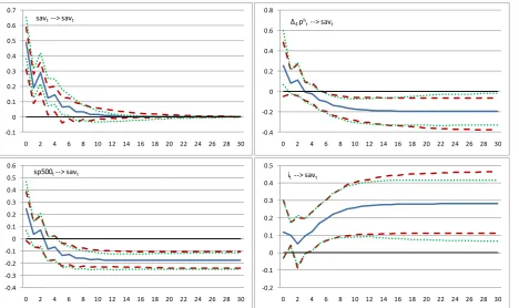
Figure 2 shows the responses of the saving ratio to a stock price, house price inflation, and mortgage rate shock together with 95% bootstrap confidence intervals based on 2000 replications over a simulation period of 30 quarters. The signs of the dynamic responses are exactly as we expected theoretically. A positive saving ratio shock has a significant positive impact on itself for about two years. In the long run there is no significant effect, which is in line with the restriction applied to the long-run matrix. A positive stock price shock, instead, leads to an initial positive reaction of the saving rate, but it is not statistically significant. The effect on the saving ratio becomes negative and significant only after about four quarters. In the long run the effect remains significant. Similar considerations apply to a positive shock to house price inflation. Finally, the saving ratio increases after a shock to the mortgage rate. This effect becomes significant after about 4 quarters.

(Figure 2 here)

Overall, IRF analysis suggests that: (a) asset prices and mortgage rate shocks have an impact on saving with some delay; (b) MEW shocks (through their component house prices and mortgage rates) exert an important impact on saving, confirming that the MEW effect has played an important role in saving during the last 20 years.

III Conclusions

We investigated the personal saving ratio in the US economy for the period of the last two decades, a period characterized by a huge decline in saving. We found that the two variables explaining the MEW mechanism (house price inflation and mortgage rate) enter a long-run relationship of the saving ratio together with the stock price. We tested the cointegrating relationship using the VEC approach. We then estimated a structural form imposing restrictions on the long-run impact matrix. All the restrictions used are justifiable by theoretical or empirical models presented in the literature. Impulse responses show that the saving ratio responds negatively to asset price shocks and positively to mortgage rate shocks according to the theory.

5

However, we have proved that the position can be changed between sp500 and and the results do not

Our analysis confirms that the variables explaining MEW have an important role, together with the stock price, in explaining the dynamic of the personal saving ratio in the last 20 years.

References

Bernanke, B. S., and Gertler, M. 1999. Monetary policy and asset price volatility. Federal Reserve Bank of Kansas City Economic Review 4: 17–53.

Deep, A., and Domanski, D. 2002. Housing markets and economic growth: Lessons from the U.S. refinancing boom. BIS Quarterly Review: 37–45.

Gonzalo, J. 1994. Five alternative methods of estimating long-run equilibrium relationships. Journal of Econometrics 60: 203–233.

Greenspan, A., and Kennedy, J. 2008. Sources and uses of equity extracted from homes. Oxford Review of Economic Policy 24: 120–144.

Guidolin, M., and La Jeunesse 2007. The decline of the U.S. personal saving rate: Is it real and is it a puzzle?

Federal Reserve Bank of St. LouisReview 89: 491–514.

Hatzius, J. 2006. Housing holds the key to Fed policy. Global Economics Paper No. 37, Goldman Sachs.

Johansen, S. 1995. Likelihood-based inference in cointegrated vector autoregressive models. Oxford: Oxford University Press.

Juselius, K. 2001. Big shocks, outliers and interventions. A cointegration and common trends analysis of daily bond rates. Mimeo, European University Institute, Florence.

Juselius, K. 2006. The cointegrated VAR model: Methodology and applications. Oxford: Oxford University Press.

Leamer, E. E. 2008. Housing is the business cycle. Proceedings, Federal Reserve Bank of Kansas City: 359–

413.

Mehra, Y. P. 1996. Monetary policy and long-term interest rates. Federal Reserve Bank of Richmond Economic Quarterly 82: 27–49.

Lutkepohl, L., and Kratzick, M. 2004. Applied time series econometrics. Cambridge: Cambridge University Press.

Saikkonen, P., and Lutkepohl, H. 2000. Testing for cointegrating rank of a VAR process with an intercept.

Econometric Theory 16: 373–406.

A. Paradiso -25 -20 -15 -10 -5 0 5 10 15 20 1 9 8 8 Q 1 1 9 8 9 Q 1 1 9 9 0 Q 1 1 9 9 1 Q 1 1 9 9 2 Q 1 1 9 9 3 Q 1 1 9 9 4 Q 1 1 9 9 5 Q 1 1 9 9 6 Q 1 1 9 9 7 Q 1 1 9 9 8 Q 1 1 9 9 9 Q 1 2 0 0 0 Q 1 2 0 0 1 Q 1 2 0 0 2 Q 1 2 0 0 3 Q 1 2 0 0 4 Q 1 2 0 0 5 Q 1 2 0 0 6 Q 1 2 0 0 7 Q 1 2 0 0 8 Q 1 2 0 0 9 Q 1 2 0 1 0 Q 1

Δ4ph

0 2 4 6 8 10 12 1 9 8 8 Q 1 1 9 8 9 Q 1 1 9 9 0 Q 1 1 9 9 1 Q 1 1 9 9 2 Q 1 1 9 9 3 Q 1 1 9 9 4 Q 1 1 9 9 5 Q 1 1 9 9 6 Q 1 1 9 9 7 Q 1 1 9 9 8 Q 1 1 9 9 9 Q 1 2 0 0 0 Q 1 2 0 0 1 Q 1 2 0 0 2 Q 1 2 0 0 3 Q 1 2 0 0 4 Q 1 2 0 0 5 Q 1 2 0 0 6 Q 1 2 0 0 7 Q 1 2 0 0 8 Q 1 2 0 0 9 Q 1 2 0 1 0 Q 1 imtg 0 200 400 600 800 1000 1200 1400 1600 1 9 8 8 Q 1 1 9 8 9 Q 1 1 9 9 0 Q 1 1 9 9 1 Q 1 1 9 9 2 Q 1 1 9 9 3 Q 1 1 9 9 4 Q 1 1 9 9 5 Q 1 1 9 9 6 Q 1 1 9 9 7 Q 1 1 9 9 8 Q 1 1 9 9 9 Q 1 2 0 0 0 Q 1 2 0 0 1 Q 1 2 0 0 2 Q 1 2 0 0 3 Q 1 2 0 0 4 Q 1 2 0 0 5 Q 1 2 0 0 6 Q 1 2 0 0 7 Q 1 2 0 0 8 Q 1 2 0 0 9 Q 1 2 0 1 0 Q 1 S&P500 0 1 2 3 4 5 6 7 8 1 9 8 8 Q 1 1 9 8 9 Q 1 1 9 9 0 Q 1 1 9 9 1 Q 1 1 9 9 2 Q 1 1 9 9 3 Q 1 1 9 9 4 Q 1 1 9 9 5 Q 1 1 9 9 6 Q 1 1 9 9 7 Q 1 1 9 9 8 Q 1 1 9 9 9 Q 1 2 0 0 0 Q 1 2 0 0 1 Q 1 2 0 0 2 Q 1 2 0 0 3 Q 1 2 0 0 4 Q 1 2 0 0 5 Q 1 2 0 0 6 Q 1 2 0 0 7 Q 1 2 0 0 8 Q 1 2 0 0 9 Q 1 2 0 1 0 Q 1 sav

Figure 1: Time series used in VEC estimation, 1988q1–2010q1

Table 1: DOLS estimates of active MEW

Model amewt/ydt= t

k k J h j t j k k j mtg j t j h t mtg

t p i p

i 2 4 1, 2, 4

1 0

Long-run relation amewt/ydt = 0 1itmtg 2 4pth ut

Sample Period β0 β1 β2

1991q1–2008q2 -3.744* -0.298*** 0.099***

Phillips–Ouliaris test -4.23***

Note: *, **, *** represent, respectively, the significance levels of 10%, 5%, and 1%. amew indicates the natural logarithm of AMEW. Leads and lags of DOLS estimations are selected according to HQ criteria. The sample period denotes the range of data before the data points for leads and lags are removed. Newey–West corrected t-statistics are applied in regression.

Table 2: Diagnostic tests for VAR(2) specifications

Q16 MARCHLM(5)

= 2 210.7 [0.73] 234.38 [0.30] 95.96 [0.11] 19.82 [0.01] 549.0 [0.06]

Note: p-values in brackets. = multivariate Ljiung–Box portmentau test tested up to the lag; = LM (Breusch–Godfrey) test for

autocorrelation up to the lag; = multivariate Lomnicki–Jarque–Bera test for non-normality from Lutkepohl (2004) with p variables in the

system; = multivariate LM test for ARCH up to the lag.

Table 3: Specification tests for VAR(2) model

Univariate normality test for sav sp500

Norm(2) 0.512 [0.774] 12.919 [0.00] 5.36 [0.069] 4.262 [0.119]

Skewness 0.151 -0.404 -0.215 0.51

Excess kurtosis 3.223 4.706 4.138 3.366

Table 4: Multivariate cointegration tests

Johansen cointegration test

Test statistics Critical values

H0 P = 2 90% 95% 99%

r = 0 52.29 50.50 53.94 60.81

r = 1 33.3 32.25 35.07 40.78

r = 2 16.57 17.98 20.16 24.69

r = 3 6.23 7.6 9.14 12.53

Saikkonen and Lutkepohl test

Test statistics Critical values

H0 P = 2 90% 95% 99%

r = 0 40.99 37.04 40.07 46.2

r = 1 20.34 21.76 24.16 29.11

r = 2 9.75 10.47 12.26 16.1

r = 3 0.33 2.98 4.13 6.93

Notes: Deterministic term: constant in the cointegrating relationship.

Table 5: Cointegration vector and loading parameters for VECM with two lagged differences and cointegrating rank r =1

s&p500 sav constant

-1.6 (3.6) -0.042 (2.1) 0.469 (2.9) 1 11.48 (2.87) -0.014 (1.78) -0.276 (1.86) - -0.404 (5.25)

Note: t-statistics in parentheses. Top-down subset restrictions exclude loading factor from mortgage rate.

Figure 2: Impulse response analysis

-0.1 0 0.1 0.2 0.3 0.4 0.5 0.6 0.7

0 2 4 6 8 10 12 14 16 18 20 22 24 26 28 30

savt--> savt

-0.4 -0.2 0 0.2 0.4 0.6 0.8

0 2 4 6 8 10 12 14 16 18 20 22 24 26 28 30

Δ4 pht--> savt

-0.4 -0.3 -0.2 -0.1 0 0.1 0.2 0.3 0.4 0.5 0.6

0 2 4 6 8 10 12 14 16 18 20 22 24 26 28 30

sp500t--> savt

-0.2 -0.1 0 0.1 0.2 0.3 0.4 0.5

0 2 4 6 8 10 12 14 16 18 20 22 24 26 28 30