Munich Personal RePEc Archive
Capital Structure Decisions: Which
Factors are Reliably Important?
Frank, Murray Z. and Goyal, Vidhan K.
University of Minnesota, Hong Kong University of Science and
Technology
1 January 2009
This is the pre-peer-reviewed version of the following article: Frank, Murray, and Vidhan K. Goyal, 2009. “Capital structure decisions: Which factors are reliably important?”' Financial Management 38, 1-37. It has been published in final form at:
http://www3.interscience.wiley.com/journal/122368692/issue
Capital Structure Decisions:
Which Factors are Reliably Important?
Murray Z. Frank and Vidhan K. Goyal
*ABSTRACT
This paper examines the relative importance of many factors in the capital structure decisions of publicly traded American firms from 1950 to 2003. The most reliable factors for explaining market leverage are: median industry leverage (+ effect on leverage), market-to-book assets ratio (-), tangibility (+), profits (-), log of assets (+), and expected inflation (+). In addition, we find that dividend-paying firms tend to have lower leverage. When considering book leverage, somewhat similar effects are found. However, for book leverage, the impact of firm size, the market-to-book ratio, and the effect of inflation are not reliable. The empirical evidence seems reasonably consistent with some versions of the tradeoff theory of capital structure.
JEL classification: G32
Keywords: Capital structure, Pecking order, Tradeoff theory, market timing, multiple imputation.
We thank Werner Antweiler, Michael Barclay, William Christie, Sudipto Dasgupta, John Graham, Keith Head, Kai Li, William Lim, Michael Lemmon, Ernst Maug, Vojislav Maksimovic, Ron Masulis, Jay Ritter, Sheridan Titman, Ivo Welch, Jeff Wurgler; seminar participants at the Tulane University and the Queen's University; participants at the 2004 American Finance Association Meetings and the 2004 NTU International Conference; and especially our anonymous referees for helpful comments. Murray Z. Frank thanks Piper Jaffray for financial support. Vidhan K. Goyal thanks the Research Grants Council of Hong Kong (Project number: HKUST6489/06H) for financial support.
*
Murray Z. Frank, Carlson School of Management, University of Minnesota, Minneapolis, MN
55455. E-mail: murra280@umn.edu. Vidhan K. Goyal, Department of Finance, Hong Kong
When corporations decide on the use of debt finance, they are reallocating some expected
future cash flows away from equity claimants in exchange for cash up front. The factors that
drive this decision remain elusive despite a vast theoretical literature, and despite decades of
empirical tests. This stems in part from the fact that many of the empirical studies are aimed at
providing support for a particular theory. The amount of evidence is large, and so it is often all
too easy to provide some empirical support for almost any idea. This is fine for a given paper,
but more problematic for the overall development of our understanding of capital structure
decisions. As a result, in recent decades the literature has not had a solid empirical basis to
distinguish the strengths and the weaknesses of the main theories.
Which theories shall we take seriously? Naturally, opinions differ. Many theories of capital
structure have been proposed. But only a few seem to have many advocates. Notably, most
corporate finance textbooks point to the “tradeoff theory” in which taxation and deadweight
bankruptcy costs are key. Myers (1984) proposed the “pecking order theory” in which there is a
financing hierarchy of retained earnings, debt and then equity. Recently the idea that firms
engage in “market timing” has become popular. Finally, agency theory lurks in the background
of much theoretical discussion. Agency concerns are often lumped into the tradeoff framework
broadly interpreted.
Advocates of these models frequently point to empirical evidence to support their preferred
study by Titman and Wessels (1988).1 These two classic papers illustrate a serious empirical
problem. They disagree over basic facts.
According to Harris and Raviv (1991, p. 334), the available studies “generally agree that
leverage increases with fixed assets, non-debt tax shields, growth opportunities, and firm size
and decreases with volatility, advertising expenditures, research and development expenditures,
bankruptcy probability, profitability and uniqueness of the product.” However, Titman and
Wessels (1988, p. 17) find that their “results do not provide support for an effect on debt ratios
arising from non-debt tax shields, volatility, collateral value, or future growth.” Consequently,
advocates of particular theories are offered a choice of diametrically opposing well-known
summaries of “what we all know” from the previous literature. Clearly this is unsatisfactory, and
this study aims to help resolve this empirical problem.
This paper contributes to our understanding of capital structure in several ways. First, starting
with a long list of factors from the prior literature, we examine which factors are reliably signed,
and reliably important, for predicting leverage. Second, it is likely that patterns of corporate
financing decisions have changed over the decades. During the 1980s, many U.S. firms took on
extra leverage apparently due to pressure from the market for corporate control. Starting in the
1990s, more small firms made use of publicly traded equity. It is therefore important to examine
the changes over time. Finally, it has been argued that different theories apply to firms under
1
different circumstances.2 To address this serious concern, the effect of conditioning on firm
circumstances is studied.
In testing which factors are correlated with leverage, it is necessary to define leverage. Many
different empirical definitions have been used. Some scholars advocate book leverage, while
others advocate market leverage. The opinions on which is a better measure of leverage differ.
According to Myers (1977), managers focus on book leverage because debt is better supported
by assets in place than it is by growth opportunities. Book leverage is also preferred because
financial markets fluctuate a great deal and managers are said to believe that market leverage
numbers are unreliable as a guide to corporate financial policy. Consistent with the academic
perception of manager's views, in Graham and Harvey (2001), a large number of managers
indicate that they do not rebalance their capital structure in response to equity market movements.
The presence of adjustment costs prevent firms from rebalancing continuously.3
Advocates of market leverage argue that the book value of equity is primarily a ‘plug number’
used to balance the left-hand side and the right-hand side of the balance sheet rather than a
managerially relevant number (see, for example, Welch (2004)). Welch further objects that the
book value of equity can even be negative (although assets cannot be). The book measure is
backward looking. It measures what has taken place. Markets are generally assumed to be
forward looking. Thus, there is no reason why these two measures should match (see Barclay,
Morellec, and Smith (2006)). The literature also uses different definitions of debt. Debt can be
2
“There is no universal theory of capital structure, and no reason to expect one. There are useful conditional theories, however. … Each factor could be dominant for some firms or in some circumstances, yet unimportant elsewhere” (Myers, 2003, pp. 216-217).
3
defined as long-term or total debt, and it can be defined to include accounts payable or all
liabilities.
In presenting our results, our main focus is on the ratio of total debt to market value of assets
(TDM). However, given these differing views, we also report results for alternative definitions of
leverage. We do find reliable empirical patterns that account for much of the variation in market
leverage across firms using a sample of publicly traded U.S. firms from 1950-2003.4 With a
market-based definition of leverage, we find that a set of six factors account for more than 27%
of the variation in leverage, while the remaining factors only add a further 2%. We call this set of
six factors “core factors” and the model that includes these factors the “core model of leverage”.
The core factors have consistent signs and statistical significance across many alternative
treatments of the data. The remaining factors are not nearly as consistent. The core factors for the
market leverage are as follows.
Industry median leverage: Firms in industries in which the median firm has high
leverage tend to have high leverage.
Tangibility: Firms that have more tangible assets tend to have higher leverage.
Profits: Firms that have more profits tend to have lower leverage.
Firm size: Firms that are large (in terms of assets) tend to have higher leverage.
Market-to-book assets ratio: Firms that have a high market-to-book ratio tend to have
lower leverage.
4
Expected inflation: When inflation is expected to be high, firms tend to have high
leverage.
This set of core factors raises several important questions. (1) Are all of these effects equally
reliable? (2) Can we replace some of the core factors with other common factors and still
adequately control for the known facts? (3) How important are the excluded factors? (4) How
does this set of core factors relate to the popular theories of leverage?
Question 1. Of course, these factors are not all equally reliable. Expected inflation is likely to
be the least reliable factor. It is the only macroeconomic factor to be included and so instead of
having over 270,000 firm-year observations, we have just 54 annual observations for expected
inflation. Accordingly, we cannot have nearly the same level of confidence that this factor will
perform similarly out of sample.
The six core factors provide a more powerful account of a market-based definition of
leverage than of a book-based definition of leverage. If we had been focusing on a book-based
definition of leverage, the market-to-book ratio, firm size and expected inflation would all have
been excluded from the core model. The remaining factors, i.e., industry median leverage,
tangibility, and profits are robust across various alternative definitions of leverage.
Recall that market-based leverage is forward looking, while book-based leverage is backward
looking. From this point of view, it would appear that the market-to-book, firm size, and
expected inflation factors are reflecting effects that are forward looking. The industry median,
There have been significant changes in the core model over time. The most important of
these is the declining importance of profits. In the period before the 1980s, profits played a very
powerful role in determining leverage. In the later period, profits – while still statistically
significant – became less important in leverage decisions. This result provides yet more evidence
of the fact, discussed in Frank and Goyal (2003), that during the 1980s and 1990s, equity
markets became more willing to fund currently unprofitable firms with good growth prospects.
When we consider firms in different circumstances, the most important fact is the degree of
similarity among the factors. However, as should be expected, there are interesting differences to
be found. The most noteworthy difference is between high and low market-to-book firms.
Tangibility and firm size are more important in explaining leverage for low market-to-book firms
than they are for high market-to-book firms.
Question 2. Many studies in the literature have used different sets of factors. Three variations
on the list of six factors are likely to be innocuous. First, replacing assets with sales is unlikely to
matter, since both reflect the role of firm size. Second, replacing expected inflation with the
nominal Treasury bill rate is unlikely to matter since they are highly correlated. Third, replacing
tangibility with collateral is unlikely to matter. Tangibility and collateral differ in that collateral
includes inventories while tangibility does not. Inventories usually support short-term debt. In
addition, inventories as a fraction of total assets have declined significantly over time.
When selecting control factors, some studies point to the four factors used by Rajan and
Zingales (1995). Their factors are: market-to-book, profit, tangibility, and sales. These factors
are reasonable but this list excludes the effect of expected inflation and median industry leverage.
regressions. We show that these omissions can materially change inferences on other factors that
are included in the model. The included minor factors sometimes become insignificant or, even
worse, change sign when the set of core factors is changed.
Question 3. Statistically, the excluded factors make little difference. As mentioned above,
they add little to the explanatory power of the model and many of them have effects that are not
reliable. On the other hand, these factors may be critical for the consideration of particular
theories. For this reason we also report the patterns that are observed for the minor factors.
Question 4. The current paper does not provide structural tests of capital structure theories.
Instead, the focus is on identifying reliable patterns in the data. If a factor is known to be reliably
related to leverage decade after decade, then a useful theory ought to be able to account for that
fact. Often the theories make specific predictions about the signs of the coefficients that should
be observed. We therefore consider the extent to which some aspects of the evidence pose
problems for theory. Using this information, we offer suggestions about directions in which the
theories might be developed so they can be more empirically relevant.
Five of the six core factors have the sign predicted by the static tradeoff theory in which
deadweight bankruptcy costs are traded-off against the tax saving of debt. The sign on profits is
inconsistent with the static tradeoff theory, but is consistent with dynamic tradeoff models such
as Fischer, Heinkel, and Zechner (1989) in which firms allow their leverage to drift most of the
time, and only adjust their leverage if it gets too far out of line.5 It is similarly consistent with
5
Tsyplakov (2008) in which, due to time-to-build, firms stock-pile retained earnings until the time
is right to buy physical capacity.
While the tax versus bankruptcy tradeoff is the most common version of the tradeoff theory,
it is not the only model within the general tradeoff theory label. Tradeoff theory also includes
models such as Stulz (1990) and Morellec (2004) in which agency costs play a crucial role. In
Stulz (1990), for example, financing policies matter because they influence the resources under
manager's control. This reduces the costs of over- and under-investment. We suspect that agency
costs of managerial discretion and stockholder-bondholder conflicts are likely quite important
relative to taxes. Our findings reproduce the well-known fact that tax effects are relatively hard
to clearly identify in the data. Even if taxes are not the full story, they matter at least to some
extent (see Graham (2003)). In addition, Hennessy and Whited (2005) show that due to
transactions costs, it is possible that tax effects will be hard to identify empirically even when
they are an element of the firm's problem. For these reasons, we think that distinguishing the
relative importance of the agency costs versus the tax-bankruptcy costs tradeoffs deserves further
work.
The pecking order theory is often used to explain financing decisions of firms. A significant
merit of the pecking order theory is that it predicts the effect of profits correctly (Shyam-Sunder
and Myers (1999)). However, as shown by Fama and French (2002) and Frank and Goyal (2003),
the theory has other problems.6 In its current form, the pecking order theory is not helpful in
organizing many of the features we see in the way firms finance themselves.
6
The market timing theory makes correct predictions for the market-to-book assets ratio and
the effect of expected inflation. However, by itself market timing does not make any predictions
for many of the patterns in the data that are accounted for by the tradeoff theory. The market
timing theory needs considerable theoretical development to explain all of empirical regularities
we observe in the data.
There is no unified model of leverage currently available that can directly account for the six
reliable factors. However, the main elements that might be used to create such a theory are
present in the literature already. The theory will have to be explicitly inter-temporal to reflect the
effects of market-to-book and expected inflation. To reflect profits, the theory is likely to have a
friction such as significant fixed costs of adjustment or time-to-build. To capture the role of
tangibility, it will need to have some role for repossession of assets by the suppliers of debt. The
theory might well have a role for financial constraints of some type to explain the effect of firm
size.
The rest of this paper is organized as follows. We provide a brief overview of the main
prediction of leading capital structure theories in Section I. The data are described in Section II.
The factor selection process and results are presented in Section III. This leads to the core model
of leverage that is presented in Section IV. The conclusions are presented in Section V.
I.
Capital
structure
theories
and
their
predictions
This section provides a brief review of the prominent theories of capital structure followed by
a summary of predictions on how the theories relate to observable leverage factors. A more
A. Capital structure theories
1. Tradeoff theory
According to the tradeoff theory, capital structure is determined by a tradeoff between the
benefits of debt and the costs of debt. The benefits and costs can be obtained in a variety of ways.
The “tax-bankruptcy tradeoff” perspective is that firms balance the tax benefits of debt against
the deadweight costs of bankruptcy. The “agency” perspective is that debt disciplines managers
and mitigates agency problems of free cash flow since debt must be repaid to avoid bankruptcy
(Jensen and Meckling (1976) and Jensen (1986)). Although debt mitigates shareholder-manager
conflicts, it exacerbates shareholder-debtholder conflicts (Stulz (1990)).
Product and factor market interactions suggest that in some firms, efficiency requires a firm's
stakeholders to make significant firm-specific investments. Capital structures that make these
firm-specific investments insecure will generate few such investments. Theory suggests that
capital structure could either enhance or impede productive interactions among the stakeholders.
Titman (1984) argues that firms making unique products will lose customers if they appear likely
to fail. Maksimovic and Titman (1991) consider how leverage affects a firm's incentives to offer
a high quality product. Jaggia and Thakor (1994) and Hart and Moore (1994) consider the
importance of managerial investments in human capital. These perspectives differ from the
tax-bankruptcy tradeoff in that the costs of debt are from disruption to normal business operations
and thus do not depend on the arguably small direct costs of bankruptcy. In other words, the
product and factor market interaction based tradeoff theories can be viewed as trading off the
2. Pecking order theory
While the pecking order theory has long roots in the descriptive literature, it was clearly
articulated by Myers (1984). Consider three sources of funds available to firms – retained
earnings, debt, and equity. Equity has serious adverse selection, debt has only minor adverse
selection, and retained earnings avoid the problem. From the point of view of an outside investor,
equity is strictly riskier than debt. Rational investors will thus revalue a firm's securities when it
announces a security issue. For all but the lowest quality firm, the drop in valuation of equity
makes equity look undervalued, conditional on issuing equity. From the perspective of those
inside the firm, retained earnings are a better source of funds than outside financing. Retained
earnings are thus used when possible. If retained earnings are inadequate, debt financing will be
used. Equity is used only as a last resort. This is a theory of leverage in which there is no notion
of an optimal leverage ratio. Although the pecking order theory is almost always framed in terms
of asymmetric information, it can also be generated from tax, agency or behavioral
considerations.7
3. Market timing theory
Market timing, a relatively old idea (see Myers (1984)), is having a renewed surge of
popularity in the academic literature. In surveys, such as those by Graham and Harvey (2001),
managers continue to offer at least some support for the idea. Consistent with market timing
behavior, firms tend to issue equity following a stock price run-up. In addition, studies that
analyze long-run stock returns following corporate financing events find evidence consistent
7
with market timing.8 Lucas and McDonald (1990) analyze a dynamic adverse selection model
that combines elements of the pecking order with the market timing idea, which can explain
pre-issue runups but not post-pre-issue underperformance. Baker and Wurgler (2002) argue that capital
structure is best understood as the cumulative effect of past attempts to time the market.
The basic idea is that managers look at current conditions in both debt and equity markets. If
they need financing, they use whichever market currently looks more favorable. If neither market
looks favorable, they may defer issuances. Alternatively, if current conditions look unusually
favorable, funds may be raised even if the firm has no need for funds currently.
While this idea seems plausible, it has nothing to say about most of the factors traditionally
considered in studies of corporate leverage. However, it does suggest that stock returns and debt
market conditions will play an important role in capital structure decisions.
B. Predictions
From the existing literature, we extract a long list of factors claimed to have some influence
on corporate leverage. This list includes measures of profitability, size, growth, industry, nature
of assets, taxation, risk, supply-side constraints, stock market conditions, debt market conditions,
and macroeconomic conditions.9 Appendix A provides a description of these factors. The
8
The evidence that equity issuers have low subsequent abnormal returns shows up in a number of studies (see, for example, Loughran and Ritter (1995) and Jegadeesh (2000)). Furthermore, Baker and Wurgler (2000) find low returns on the stock market following heavy aggregate stock issuance.
9
theories are not developed in terms of standard accounting definitions. To test the theories, it is
therefore necessary to make judgments about the connection between the observable data and
theory. While many of these judgments seem uncontroversial, there is room for significant
disagreement in some cases.
1. Leverage and profitability
Profitable firms face lower expected costs of financial distress and find interest tax shields
more valuable. Thus, the tax and the bankruptcy costs perspective predicts that profitable firms
use more debt. In addition, the agency costs perspective predicts that the discipline provided by
debt is more valuable for profitable firms as these firms are likely to have severe free cash flow
problems (Jensen (1986)).
Recent papers, however, suggest that the tradeoff theory predictions on profitability are more
complex than those based on static models (see Strebulaev (2007)). In a dynamic trade-off model,
leverage can appear to be negatively related to profitability in the data due to various frictions.
Empirically, the response has been to argue that leverage and profitability are negatively related
because firms passively accumulate profits (see Kayhan and Titman (2007)).10
The pecking order theory argues that firms prefer internal finance over external funds. If
investments and dividends are fixed, then more profitable firms will become less levered over
time.
Measure: Profitability
10
2. Leverage and firm size
Large, more diversified, firms face lower default risk. In addition, older firms with better
reputations in debt markets face lower debt-related agency costs. Thus, the tradeoff theory
predicts larger, more mature firms to have relatively more debt.
The pecking order theory is usually interpreted as predicting an inverse relation between
leverage and firm size and between leverage and firm age. Large firms are better known as they
have been around longer. In addition, older firms have had an opportunity to retain earnings.
Measures: (i) Log of assets, and (ii) Mature firms
3. Leverage and growth
Growth increases costs of financial distress, reduces free cash flow problems, and
exacerbates debt-related agency problems.11 Growing firms place a greater value on stakeholder
co-investment. Thus, the tradeoff theory predicts that growth reduces leverage.
By contrast, the pecking order theory implies that firms with more investments - holding
profitability fixed - should accumulate more debt over time. Thus, growth opportunities and
leverage are positively related under the pecking order theory.
The market-to-book asset ratio is the most commonly used proxy for growth opportunities.
Adam and Goyal (2008) show that it is also the most reliable. A higher market-to-book ratio,
however, may also be influenced by stock mispricing. If market timing drives capital structure
decisions, a higher market-to-book ratio should reduce leverage as firms exploit equity
11
mispricing through equity issuances. Furthermore, a mechanical negative relation may exist
between a market-based definition of leverage and the market-to-book-assets ratio.
Capital expenditures and the change in log assets, which are also proxies for growth,
represent outflows. They directly increase the financing deficit as discussed in Shyam-Sunder
and Myers (1999). These variables should therefore be positively related to debt under the
pecking order theory.
Measures: (i) the market to book ratio, (ii) Change in log assets, and (iii) Capital expenditure to
assets ratio
4. Leverage and industry conditions
It is well known that leverage ratios exhibit significant variation across industries. Textbooks
in corporate finance such as Ross, Westerfield, and Jaffe (2008) routinely point to inter-industry
differences in debt ratios. More formal tests are presented in Lemmon, Roberts, and Zender
(2008). Industry differences in leverage ratios have several possible meanings. One interpretation
is that managers perhaps use industry median leverage as a benchmark as they contemplate their
own firm's leverage. Thus, industry median leverage is often used as a proxy for target capital
structure (see, for example, Gilson (1997), Hull (1999), Hovakimian, Opler, and Titman (2001),
Faccio and Masulis (2005), and Flannery and Rangan (2006)). Hovakimian, Opler, and Titman
(2001) provide evidence consistent with firms actively adjusting their debt ratios towards the
Another interpretation is that industry effects reflect a set of correlated, but otherwise omitted
factors.12 Firms in an industry face common forces that affect their financing decisions. These
could reflect product market interactions or the nature of competition.13 These could also reflect
industry heterogeneity in the types of assets, business risk, technology, or regulation. Industry
factors do not have a unique interpretation.
We consider two industry variables – industry median growth and industry median leverage.
Tradeoff theory predicts that higher industry median growth should result in less debt, while
higher industry median leverage should result in more debt. Finally, we consider if firms are
regulated. Regulated firms have stable cash flows and lower expected costs of financial distress.
Thus, regulated firms should have more debt. But, at the same time, managers have less
discretion in regulated firms, which reduces the severity of shareholders-managers conflicts and
makes debt less desirable from a control perspective. Tradeoff theory makes an ambiguous
prediction on the effect of regulation on leverage.
Under a pure pecking order perspective, the industry should only matter to the extent that it
serves as a proxy for the firm's financing deficit - a rather indirect link. Under the market timing
theory, the industry should matter only if valuations are correlated across firms in an industry.
Measures: (i) Median industry leverage, (ii) Median industry growth, and (iii) Regulated dummy
12
Hovakimian, Hovakimian, and Tehranian (2004) follow this interpretation and include industry leverage to control for omitted factors. It is also possible to give industry a more structural interpretation. Almazan and Molina (2005) and Mackay and Phillips (2005) interpret industry in terms of relatively specialized industry equilibrium models.
13
5. Leverage and nature of assets
Tangible assets, such as property, plant, and equipment are easier for outsiders to value than
intangibles such as the value of goodwill from an acquisition – this lowers expected distress
costs. In addition, tangibility makes it difficult for shareholders to substitute high-risk assets for
low-risk ones. The lower expected costs of distress and fewer debt-related agency problems
predict a positive relation between tangibility and leverage. An analogous prediction is that firms
making large discretionary expenditures such as SG&A expenses and R&D expenses have more
intangible assets and consequently less debt.
Stakeholder co-investment theory suggests that firms producing unique products (such as
durable goods) should have less debt in their capital structure (Titman (1984)). Firms in unique
industries have more specialized labor, which results in higher financial distress costs and
consequently less debt. To protect unique assets that result from large expenditures on SG&A
and R&D, these firms will have less debt.
The pecking order theory makes opposite predictions. Low information asymmetry
associated with tangible assets makes equity issuances less costly. Thus, leverage ratios should
be lower for firms with higher tangibility. However, if adverse selection is about assets in place,
tangibility increases adverse selection and results in higher debt. This ambiguity under the
pecking order theory stems from the fact that tangibility can be viewed as a proxy for different
economic forces. Furthermore, R&D expenditures increase the financing deficit. R&D
expenditures are particularly prone to adverse selection problems and affect debt positively under
Measures: (i) Tangibility, (ii) R&D expense/sales, (iii) Uniqueness dummy, and (iv) selling,
general and administrative expense/sales ratio.
6. Leverage and taxes
High tax rates increase the interest tax benefits of debt. The tradeoff theory predicts that to
take advantage of higher interest tax shields, firms will issue more debt when tax rates are higher.
Deangelo and Masulis (1980) show that non-debt tax shields are a substitute for the tax benefits
of debt financing. Non-debt tax shield proxies i.e. net operating loss carryforwards, depreciation
expense, and investment tax credits – should be negatively related to leverage.
Measures: (i) Top tax rate, (ii) NOL carry forwards/assets, (iii) Depreciation/assets, and (iv)
Investment tax credit/assets
7. Leverage and risk
Firms with more volatile cash flows face higher expected costs of financial distress and
should use less debt. More volatile cash flows reduce the probability that tax shields will be fully
utilized. Risk is detrimental for stakeholder co-investment. Thus higher risk should result in less
debt under the tradeoff theory.
We might expect firms with volatile stocks to be those about which beliefs are quite volatile.
It seems plausible that such firms suffer more from adverse selection. If so, then the pecking
order theory would predict that riskier firms have higher leverage. Also, firms with volatile cash
flows might need to periodically access the external capital markets.
8. Leverage and supply-side factors
Faulkender and Petersen (2006) argue that supply-side factors are important in explaining the
variation in capital structure. When firms have restricted access to debt markets, all else equal,
financing takes place through equity markets. Less debt is issued because of restricted debt
market access. The proxy they use for access to debt markets is whether the firm has rated debt.
Firms with a debt rating are expected to have more debt, ceteris paribus.
From a pecking order perspective, however, possessing a credit rating involves a process of
information revelation by the rating agency. Thus, firms with higher ratings have less of an
adverse selection problem. Accordingly, firms with such ratings should use less debt and more
equity. But this is ambiguous, since less adverse selection risk increases the frequency with
which the external capital market is accessed, which would result in more debt.
Measures: Debt rating dummy
9. Leverage and stock market conditions
Welch (2004) argues that firms do not re-balance capital structure changes caused by stock
price shocks and therefore stock returns are “considerably more important in explaining
debt-equity ratios than all previously identified proxies together.”' Market timing theories make
similar predictions but the effects come from managers actively timing equity markets to take
advantage of mispricing. Time-varying adverse selection could also result in a negative relation
between stock prices and leverage. Choe, Masulis, and Nanda (1993) show that at the aggregate
level, seasoned equity issues are pro-cyclical while debt issues are counter-cyclical. Korajczyk,
firms issue equity following price run-ups. In summary, the effect of stock prices on leverage
could reflect (i) growth (as discussed previously), (ii) changes in the relative prices of asset
classes (reflecting changes in aggregate conditions), (iii) market timing (reflecting changes in
firm-specific conditions), and (iv) changes in adverse selection costs. The prediction that strong
market performance results in a reduction in market leverage could be derived from any of the
leading capital structure theories. Static tradeoff models would predict that low market debt
ratios ought to encourage a company to issue debt in an attempt to move towards the optimum,
which would have the effect of raising book debt ratios following high stock returns. The market
timing theory, on the other hand, makes the contrary prediction that book debt ratios should fall
following high stock returns as firms issue equity.
Measures: (i) Cumulative raw returns, and (ii) Cumulative market returns
10.Leverage and debt market conditions
According to Taggart (1985), the real value of tax deductions on debt is higher when
inflation is expected to be high. Thus, the tradeoff theory predicts leverage to be positively
related to expected inflation. Market timing in debt markets also results in a positive relation
between expected inflation and leverage if managers issue debt when expected inflation is high
relative to current interest rates.14 Barry et al. (2008) find that firms issue more debt when current
interest rates are low relative to historical levels.
14
The term spread is considered a credible signal of economic performance and expected
growth opportunities. If a higher term spread implies higher growth, then term spread should
negatively affect leverage.
Measures: Expected inflation rates, Term spread
11.Leverage and macroeconomic conditions
Gertler and Gilchrist (1993) show that subsequent to recessions induced by monetary
contractions, aggregate net debt issues increase for large firms but remain stable for small firms.
During expansions, stock prices go up, expected bankruptcy costs go down, taxable income goes
up, and cash increases. Thus, firms borrow more during expansions. Collateral values are likely
to be pro-cyclical too. If firms borrow against collateral, leverage should again be pro-cyclical.
However, agency problems are likely to be more severe during downturns as manager's
wealth is reduced relative to that of shareholders. If debt aligns managers incentives with those
of shareholders, leverage should be counter-cyclical.
If pecking order theory holds, leverage should decline during expansions since internal funds
increase during expansions, all else equal. If corporate profits have shown an increase in the
recent past, agency problems between shareholders and managers are less severe. Consequently
firms should issue less debt.
2.
Data
Description
The sample consists of U.S. firms on Compustat for the period from 1950 to 2003. The data
are annual and are converted to 1992 dollars using the GDP deflator. The stock return data are
from the Center for Research in Security Prices (CRSP) database. The macroeconomic data are
from various public databases. These sources are described in Appendix A. Financial firms and
firms involved in major mergers (Compustat footnote code AB) are excluded. Also excluded are
firms with missing book value of assets. The ratios used in the analysis are winsorized at the
0.50% level in both tails of the distribution. This serves to replace outliers and the most
extremely misrecorded data.15
A. Defining leverage
Several alternative definitions of leverage have been used in the literature. Most studies
consider some form of a debt ratio. These differ according to whether book measures or market
values are used. They also differ in whether total debt or only long term debt is considered. One
can also consider the interest coverage ratio as a measure of leverage (see Welch (2004)).16
Finally, firms have many kinds of assets and liabilities and a range of more detailed adjustments
can be made.
15
Prior to trimming, several balance sheet and cash flow statement items are recoded as zero if they were reported missing or combined with other data items in Compustat. The data are often coded as missing when a firm does not report a particular item or combines it with other data items. Table 8 of Frank and Goyal (2003) identifies variables coded as zero when reported missing or combined with other items. Winsorizing is the procedure of replacing extreme values with the value of the observations at the cutoffs. Only variables constructed as ratios are winsorized.
16
In the empirical work we study four alternative definitions of leverage: (a) the ratio of total
debt to market value of assets (TDM), (b) the ratio of total debt to book value of assets (TDA), (c)
the ratio of long term debt to market value of assets (LDM), and (d) the ratio of long-term debt to
book value of assets (LDA).17 Most studies focus on a single measure of leverage.
We take TDM to be the main focus. In the literature it is common to find claims that the
crucial results are robust to alternative leverage definitions. Having reviewed many such
robustness claims, we expected the results to be largely robust to the choice among the four
measures. In most regards, this is reassuring. But the robustness of many results to large
differences between alternative measures is sometimes troublesome. Cross-sectional tests may be
more robust to the measure used than time-series tests if macro variation can be netted out. For
example, the ratio of the market value of equity to the book value of equity soared between
1974-1982 and 1999-2000 for the median firm.
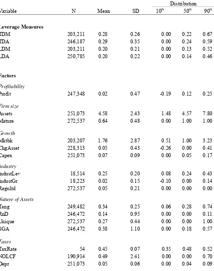
B. Descriptive Statistics
Table I provides descriptive statistics. The median leverage is below the mean leverage.
There is a large cross-sectional difference so that the 10th percentile of TDM is 0 while the 90th
percentile is 0.67. Several factors have mean values that diverge sharply from the medians.
To explore changes in U.S. corporate balance sheets and cash flow statements over time,
median balance sheets normalized by total assets for U.S. firms from 1950-2003 are presented in
Appendix Table I and median corporate cash flow statements normalized by end-of-year total
assets are presented in Appendix Table II. These tables reveal significant time-series variation in
17
the structure of balance sheets and cash flow statements of U.S. firms.18 Cash levels fell until the
1970s and then built back up. Inventories declined by almost half while net property, plant and
equipment had a more modest decline. Intangibles have become increasingly important in recent
periods. Current liabilities, especially ‘current liabilities-other’, have also increased. This
category has risen from being trivial to accounting for about 8% of the average firm's liabilities.
Long-term debt rose early in the period but has been fairly stable over the period 1970-2003. The
net effect of the various changes is that total liabilities rose from about 35% of assets to more
than 53% of assets while common book equity had a correspondingly large decline.
The changes to the cash flows are also fairly remarkable. Both sales and the cost of goods as
a fraction of assets fell dramatically. The selling, general and administrative expenses more than
doubled over the period. As a result, the median firm has negative pre-tax income by the end of
the period. Increasingly, it seems that public firms include currently unprofitable firms with
expectations of future profitability, a pattern also noted by Fama and French (2001) and
DeAngelo, DeAngelo, and Skinner (2004). We also find that corporate income taxes have
declined over time. This is not surprising since the statutory tax rates have dropped, and the
average includes more unprofitable firms. The median firm both issues and reduces a significant
amount of debt each year.
III.
Empirical
evidence
on
factor
selection
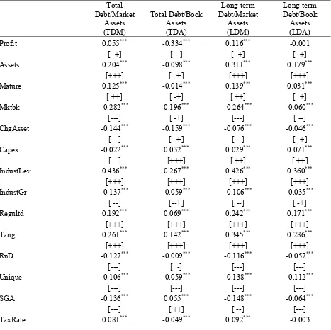
We begin by reporting the correlations between the factors and each of the leverage measures
in Table II. Beneath each correlation, the pluses and minuses indicate the fraction of the time the
correlation was of a particular sign and statistically significant at the 1% level. The sample
18
period from 1950 to 2003 is divided into six periods - the five decades and the last period
consisting of the period 2000-2003. A single + means that the correlation was positive and
significant in at least 2 out of 6 periods. A ++ means that the correlation was positive and
significant in 4 out of 6 periods. A +++ means that the correlation was positive and significant in
every period. The -, --, and ---, are analogously defined for the negative and significant cases. A
-+ indicates that the correlations are negative and significant for at least two out of six periods
and positive and significant for at least another two decades. A --+ indicates that the correlations
are negative and significant in four periods and positive and significant for the other two periods.
Similarly, a ++- indicates that the correlations are positive and significant for four periods and
negative and significant for the other two periods.
In every period, positive and significant correlations with leverage (TDM) are found for: log
of assets, median industry leverage, the dummy for being regulated, and tangibility. Similarly
powerful negative correlations are found for: the market to book ratio, research and development
expenses, uniqueness, selling general and administration expenses, the variance of stock returns,
cumulative stock returns, and term spread. With some exceptions, the factors identified here
exhibit similar correlations with the alternative leverage definitions.
Unconditional correlations are interesting, but more important are the effects of a factor when
other factors are also present in the analysis. Linear regressions are used to study the effects of
the factors. Let Li,t denote the leverage of firm i on date t. The set of factors observed at firm i at
date t-1 is denoted Fi,t-1, The constant α and the vector β are the parameters to be estimated. The
clustering on the estimated standard errors, we use t-statistics corrected for clustering at both the
firm and the year level in our tests, as suggested by Petersen (2008).19 The basic model is:
, , , . (1)
We have a long list of factors. In the interest of parsimony, it is desirable to remove
inessential factors. Hastie, Tibshirani, and Friedman (2001) describe many methods that can be
used to decide which factors to keep and which to drop. The Akaike Information Criterion (AIC)
and the Bayesian Information Criterion (BIC) are the two most commonly used model selection
criteria and we have tried both.20 Let P be the number of parameters and let N be the number of
observations in a fitted model. The Bayesian Information Criterion is defined as follows,
2 log log . (2)
The Akaike Information criterion is measured similarly, but with the number 2 replacing
log(N) in the definition. Both BIC and AIC have a sensible structure. In each case, smaller is
better. As the log-likelihood increases, both measures fall. As the number of parameters
increases, both measures increase. As the number of observations increases, so does the BIC.
BIC is asymptotically consistent. In other words, suppose that you have a family of possible
models that includes the true model. Then as the sample size grows to infinity, the probability
that the BIC will pick the true model approaches one. In small samples it is not clear whether
AIC or BIC is better. Since log (N)>2, the BIC tends to select a more parsimonious model. In our
19
We thank Petersen for the Stata ado file for two-dimensional clustering. This file can be obtained from: http://www.kellogg.northwestern.edu/faculty/petersen/htm/papers/se/se_programming.htm
20
analysis, they routinely produce the same answers. Thus, we only report the BIC. For a useful
discussion of the relative merits of many approaches to model selection, including both the AIC
and BIC, see Hastie, Tibshirani, and Friedman (2001).
Robustness of conclusions is extremely important. For this reason, in addition to overall
results, we systematically consider the results for sub-samples. Reliably important results should
be robust across sub-samples. We therefore generate 10 random sub-samples of the data and
repeat the analysis on each of these groups. We also consider annual cross-sections.
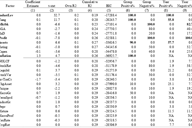
Table III presents the results of this selection process. Columns (1) to (5) illustrate the
method that generates the minimum BIC specification for the overall sample. To understand
these columns, start at the bottom of the table and estimate Equation (1) with all the factors.
Report the adjusted R2 in column (4) and the BIC in column (5). Then remove the factor with the
lowest t-statistic (in this case, it is the cumulative market return or CrspRet). Report the
coefficient estimate and the t-stat in columns (1) and (2) for the one-variable regression using
this variable. Reestimate a regression of leverage on cumulative market return and report the R2
from this regression in column (3). Next, recalculate all statistics on the reduced sample that
includes all factors except the cumulative market return. This improves the model slightly as the
BIC drops from -28,507 to -28,519. Next, remove the factor with the lowest t-statistic and
recalculate. This time it is the top tax-rate (TaxRate). This process continues removing one factor
at a time until at the top of the table only a single factor remains – the median industry
leverage.21
21
In columns (6) and (7), we randomly partition the data into 10 equal groups. The exercise to
identify the minimum BIC specification is repeated on each group separately. Under the heading
“Group Positive %” are listed the percentage of groups for which the given factor was included
in the minimum BIC specification and had the indicated sign. Similarly, “Group Negative %”
lists the percentage of groups for which the given factor was included in the minimum BIC
specification and had the indicated sign. In columns (8) and (9), we repeat the minimum BIC
selection process for each year of data run separately. Since the macro factors have only a single
observation in each year, they are excluded from the year-specific tests.
The selection of core factors is based on how often a factor is included in the minimum BIC
specification in repeated runs of the sample. To be considered, as a rule of thumb, we require a
factor to be included in at least 50% of the minimum BIC specifications. The core factors that
result from this process include (i) Industry median leverage, (2) Tangibility, (3) Market-to-book
assets ratio, (4) Profitability, (5) Log of assets, and (6) Expected inflation.22 These six factors
account for about 29% of the variation in the data. We have also examined the performance of
the variables one at a time to ensure that major variables are not being excluded from the final
model due to a quirk of path dependence in the selection process. We find no evidence of a
path-dependence problem.
which have fewer than four firms. This resulted in exclusion of roughly 1/10th of 1% of our sample. Again, the results didn't change materially.
22
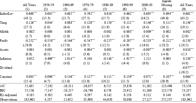
Much of the focus so far has been on a market-based definition of leverage (TDM). As
indicated earlier, this definition is frequently used in the literature, but a range of alternative
definitions have been used in other studies. The six main factors are fairly, but not perfectly,
robust. In unreported results, we find that for LDM, the robust factors would be industry median
leverage, tangibility, profitability, log of assets and the selling, general and administrative
expenses-to-sales ratio. If we consider TDA, the list includes industry median leverage,
tangibility, profitability, and net operating loss carry-forwards. If we consider LDA, the list
includes industry median leverage, tangibility, assets, profitability, and stock return variance.
Overall, we can conclude that industry median leverage, tangibility, and profitability appear as
robust factors in various definitions of leverage.
We are not aware of any theory that satisfactorily accounts for the differences that are
observed between those factors that influence the alternative definitions of leverage. It is possible
that the market-to-book assets ratio appears as a robust factor in TDM because the effect of the
market-to-book ratio may be operating through an effect on the value of equity more than
through the effect on the value of debt. There is a mechanical negative relation when market
leverage is used, but not when book leverage is used. Inflation may similarly be affecting stock
prices, thus affecting market leverage ratios more than the book leverage ratios. Ritter and Warr
(2002) argue that investors misinterpret the effects of inflation, which results in inflation-induced
valuation errors in equity markets.
A.
Financially
constrained
versus
unconstrained
firms
Myers (2003) has argued that “the theories are conditional, not general”. They work better in
some conditions than in others. The recent literature has focused on financial constraints as
Zender (2004)). We therefore examine if the factors affect leverage differently for firms that are
relatively more financially constrained. To classify firms into those that are constrained and
those that are not, we rely on dividend paying status, firm size, and the market-to-book assets
ratio. Firms that pay dividends, those that are larger and those with low growth opportunities
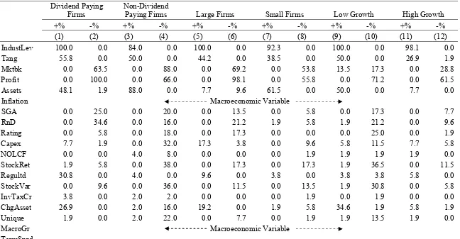
should find it relatively easy to raise external financing. Table IV presents results for
sub-samples of firms classified based on these three criteria. For each sub-sample, we repeat the
Table III exercise and then report how often the factor is included for that class of firms in
annual cross-sections. For simplicity we use a 50% cutoff rule of thumb for inclusion.
Table IV shows that none of the excluded factors should be added back to the set of six core
factors. On the other hand, some of the six included factors do not perform as well for certain
types of firms. The most important point about Table IV is the remarkable similarity of effects
across the classes of firms. Clearly, there are some differences. However, the basic patterns are
very similar for different types of firms. It seems that financing constraints at least as measured
in this manner do not have a big effect on our interpretation of the evidence.
IV.
Parameter
estimates
for
the
core
leverage
model
The analysis in Section III has provided a set of factors that are reliably important for
leverage.23 The next task is to estimate Equation (1) using the factors. Table V provides
23
parameter estimates from the core model along with t-statistics computed using standard errors
corrected for clustering both by firm and by year.24
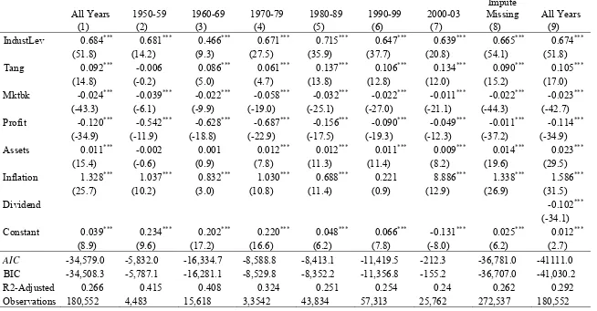
In column (1) of Table V, an overall regression model is reported that makes use of the
available data for “All Years”. In columns (2) to (7) of Table V, estimates are presented on a
decade-by-decade basis and for the four years in the 2000-2003 period. Over the decades there is
a worsening in the ability of the set of factors to explain leverage. In the 1950s, these factors
account for 42% of the variation in leverage. In the early 2000, they account for only about 24%
of the variation.25
The impact of profits declines sharply. Panel A of Table V reports that, in the 1950s, the
estimated coefficient on profitability is -0.54, while in the early 2000s, it has declined to -0.05.
This is a truly remarkable decline in the importance of profits. At the same time, the effects of
firm size and dividend paying status have both increased in economic importance.
A. Adjusting for missing data
We have so far followed standard practice in treating missing data.26 This means we have left
out the records of firms for which necessary data items are not available. Depending on what
24
Using panel regressions with either fixed effects or random effects leads to the same conclusions. This means that the factors help us to understand both the differences between firms as well as the differences for a given firm across time.
25
By way of comparison Rajan and Zingales (1995) suggest a basic model with 4 factors: tangibility, sales, market-to-book assets ratio, and profits. Their model has often been used as benchmark model (e.g., Frank and Goyal (2003)). Their four factor model does not provide as satisfactory an account of the data as these six factors. Estimates of that model account for 17.5% of the variation in the data. The biggest single missing factor is the industry effect.
26
determines which data are missing and which data are reported, biases that arise from dropping
observations with incomplete records may be important.27
The missing data problem has been well studied and it has been found that procedures,
known as “multiple imputation”, work relatively well.28 The idea of multiple imputation is to use
the facts that you can observe about a firm in a given year to predict the data that has not been
recorded. The predicted data is less certain than is the observed data. There is a distribution of
possible values. Accordingly, the standard approach is to stochastically impute the missing
values several times. In this way several data sets are created. Each data set is analyzed as if it
were a complete data set. Then the results are aggregated in order to see how sensitive the results
are to the imputed values.
The results of imputing the missing values are found in column (8) headed “Impute Missing”
in Table V.29 Imputing missing data has the effect of dramatically increasing the number of firm
years from 180,552 to 272,537.
Even with this large increase in data, for the set of factors that form the core model, it is
remarkable how little change is observed. None of the conclusions about the reliable factors are
27
To understand why this is potentially so important consider a simple example. We let x and y be two independent accounting measures that are each normally distributed with a mean of 100 and a standard deviation of 10. We generate 500 of each variable and then regress x on y. The intercept is 105 (S.E. = 4.6), the slope is -0.05 (S.E. = 0.05) and the R2=0.002. This is as it should be. Next suppose that we only include observations for which
x>100, or y>100 or both. Now the intercept is 139.9 (S.E. = 5.1) the slope is -0.37 (S.E. = 0.05) and the R2=0.12. Finally suppose that we require that x+y>200. Now the intercept is 159.9 (S.E. = 5.5) the slope is -0.52 (S.E. = 0.05) and the R2=0.27. Obviously, when there are requirements that must be satisfied in order for the data to be observed, regressions reflect both the underlying data and the data recording process.
28
The missing data problem is related to, but distinct from, the familiar survivorship bias. Compustat includes data only on firms in year t that continue to exist long enough to file an annual financial statement for year t in year t+1. This leads to the well known problem of survivorship bias. Early studies such as Titman and Wessels (1988) examined balanced panels of data. Only firms that existed over the full time period were included. In recent years this practice has been replaced by the now common use of unbalanced panels of firms. We use unbalanced panel methods.
29
affected. We have done some experimentation and found, not surprisingly, that the minor factors
are more sensitive to multiple imputation. Since we do not stress the minor factors we have not
explored this issue systematically.
B. Reintroducing the minor factors
The minor factors are of interest for some purposes. There are several reasons that justify
adding them to the core model of leverage. If a new factor materially affects the sign and
significance of one of the core factors, then it is interesting. If a new factor accounts for
significant additional variation that the factors leave unexplained, then it is interesting. If a new
factor is a variable that is policy relevant then it is interesting to add it to the model for some
purposes.
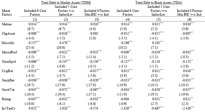
Accordingly in Table VI, we reintroduce these factors one at a time. We consider their effect
when added to the core factor model, to the five factors that exclude industry and to the eight
factors that are found robust when industry is omitted.30 We do not report coefficient estimates
on the control factors. The coefficients on the core factors are extremely stable no matter which
of the minor factors is added back in. In these regressions, the reported t-statistics use standard
errors corrected for clustering both by firm and by year.
Note that if we use conventional levels of “statistically significant”, Table VI suggests that
many of these factors are significant. This is despite the earlier evidence that these effects are
weak. This shows that it is easy to add a factor to our list and find that “it matters empirically.”
In essence, Table VI provides a lengthy list of such factors. Despite their significance, some
30
minor factors have signs that are unreliable. The choice of a leverage definition is important in
several cases. These cases may reflect either lack of robustness, or cases in which a forward
looking measure simply provides a different perspective than a backwards looking measure.
Theoretically disentangling such cases might be interesting in future work.
Table VI also presents cases where it matters whether one includes the industry factor or not.
The impact of the stock market returns, uniqueness variable, and regulated variable are reversed
depending on whether industry is included or not. The effect of stock market return on leverage
is negative and significant when industry is included, but positive and significant when it is
excluded.
Several other variables are insignificant when industry median leverage is included but
become statistically significant when it is excluded. This is important. It implies that a great deal
of robustness checking is needed to properly establish empirical results as being reliable.
As an example, consider the effect of investment tax credits. In Table II, it is positively
correlated with leverage. In Table III, it is dropped at the point where it has a coefficient of
-1.692 and a t-statistic of -3.4. What is much more interesting is seen in Table VI. Depending on
the set of factors used as controls and the definition of leverage, this factor can have either a
positive sign or a negative sign. In the market leverage regression, the t-statistic is 3.3 when
included with the core factors, but it becomes -1.2 with eight control variables: five core factors
(without industry median leverage) and three additional variables viz. dummy for regulated firm,
selling, general and administrative expense/sales ratio and macro growth. If we measure leverage
using book values, the coefficient is significantly negative regardless of the set of core factors
Adding or dropping a factor that is itself minor typically has little effect. Yet there are cases
in which one can provide “robust” evidence that a given factor has a positive sign on leverage
and yet by using a slightly different set of control factors it can also be established that the same
factor also has a robust negative effect on leverage. What this means is that using exactly the
same data, but different control factors or with different definitions of leverage, different papers
might reach different conclusions about how a particular factor relates to leverage. This is why it
is important for the literature to make use of a standardized set of control factors, such as the
robust factors.
C. Caveats
The current paper documents reliable patterns in the leverage data. We do not provide
structural tests of the theories. That is a job for another day. To mitigate concern about
endogeneity we use factors from the previous year, not contemporaneous factors. This does not
resolve the endogeneity problem nor the lack of a structural model. But at least it has the merit of
ensuring that the factors are in the firm's information set. To go further would require imposing
extra structure and then testing whether that structure fits the data. Such studies are worth doing,
but they are well outside the scope of the current paper. We hope that our results may be a useful
precursor to studies that impose more structure.
There are a number of other things that we have not studied in this paper. We have not
allowed for alternative functional forms and general non-linearities. We have not allowed for
general interaction effects, although some minor interaction effects can be found in Table IV. We
this paper.31 We have intentionally excluded firm fixed effects. Firm fixed effects are statistically
important. However, the interpretation is unclear. Their inclusion would not be appropriate for
our purposes. Including them would have its largest effect on the industry median leverage
variable. All of these are potentially interesting, and we hope to explore many of them in the
future.
V. Conclusion
This paper studies publicly traded American firms over the period 1950 to 2003 to determine
which factors have a reliable relation to market-based leverage. Starting from a large set of
factors that have been used in previous studies, we find that a set of six factors provides a solid
basic account of the patterns in the data:
Firms that compete in industries in which the median firm has high leverage tend to have high leverage.
Firms that have a high market-to-book ratio tend to have low levels of leverage.
Firms that have more tangible assets tend to have more leverage.
Firms that have more profits tend to have less leverage.
Larger firms (as measured by book assets) tend to have high leverage.
When inflation is expected to be high firms tend to have high leverage.
In addition to these six factors, a previous version of this paper finds that an indicator
variable indicating whether the firm pays a dividend is also reliably associated with leverage.
Firms that pay dividends have less leverage than nonpayers. The existing capital structure
theories have ambiguous predictions on the relation between dividend paying status and firm
leverage. In our view, the interpretation of dividends needs further development beyond that
contained in the literature.
31
Many studies report that whatever their results are, they are robust to the use of market or
book leverage. Given these past studies, we expected that the main factors would also be robust
to the choice of market or book leverage. This turns out not to be correct.
When studying book leverage, the effects of market-to-book, firm size, and expected
inflation factors all lose the reliable impact that they have when studying market-based leverage.
The industry median leverage, tangibility, and profitability remain reliable and statistically
significant.
How do we interpret this surprising finding? Recall that Barclay, Morellec, and Smith (2006)
argue book-leverage is backwards-looking while market-leverage is forwards looking. From this
perspective we see that the effects of the market-to-book assets ratio, firm size (as measured by
book assets), and expected inflation are apparently operating through their ability to capture
aspects of the firm's anticipated future. Industry median leverage, tangibility and profitability
appear to reflect the impact of the firm's past. We believe that this distinction merits future
attention from corporate finance theorists.
How good an account do these major theories provide for the main patterns we see in the
data? We study publicly traded American firms over the past half century. For these firms, the
evidence points to weaknesses in each theory – some more damaging than others. The nature of
the weaknesses differs.
Market timing is frequently pointed to by advocates of behavioral finance. But market timing
could also result from rational optimizing by managers (e.g., Baker and Wurgler (2002)). Almost
any realistic optimizing model of corporate leverage is likely to have time-varying costs and