Evaluating Aid Effectiveness in the Aggregate: Methodological Issues

Munich Personal RePEc Archive

Evaluating Aid Effectiveness in the

Aggregate: Methodological Issues

Carl-Johan, Dalgaard and Henrik, Hansen

Danida’s Evaluation Department

March 2009

Online at

https://mpra.ub.uni-muenchen.de/23025/

EVALUATING AID EFFECTIVENESS IN THE

AGGREGATE: METHODOLOGICAL ISSUES

Evaluating Aid Effectiveness in the Aggregate:

Methodological Issues

March 2009

Carl-Johan Dalgaard, Department of Economics, University of Copenhagen

Henrik Hansen, Institute of Food and Resource Economics, University of Copenhagen ____________________________________________________________

*Acknowledgement: We are grateful to Arvind Subramanian for sharing the data from Rajan and Subramanian (2008).

Disclaimer: The views expressed are those of the authors and do not necessarily represent the views of the Ministry of Foreign Affairs of Denmark. Errors and omissions are the

Contents

Executive Summary ... 3

1. Introduction ... 4

2. What is “Aid Effectiveness” at the aggregate level? ... 6

2.1. Should the focus rather be on development? ... 7

2.2. Should the focus rather be on poverty alleviation? ... 11

3. The basic empirical approach to assessing aid effectiveness: Regression analysis ... 13

4. The cause and effect problem ... 17

4.1. Simple and multiple regression analysis ... 17

4.2. Two rules colliding: The identification problem ... 19

4.3. Is it really a problem? ... 25

4.4. A possible solution to the cause and effect problem ... 28

5. An illustration of the regression approach ... 32

6. Yet another specification problem: The impact may vary ... 42

6.1. The Effect depends on the characteristics of the recipients ... 46

6.2. The Effect depends on characteristics of the donors ... 46

6.3 The regression solution: more instruments ... 47

7. Concluding remarks ... 52

Literature ... 53

Annexes ... 56

Annex 1. The Cause and Effect Problem ... 56

Annex 2. Reverse causality: the impact of growth on aid ... 58

Annex 3. Instrumental variables estimation ... 59

Executive Summary

The purpose of the present Evaluation Study is to discuss the methodological problems researchers are facing in gauging the impact of aid on economic growth. The discussion is non-technical and aimed at an audience without much prior knowledge in the fields of macroeconomics and econometrics.

The paper provides insights into the following questions:

1. Why do economists view “aid effectiveness” as synonymous to asking whether aid increases growth in income per capita?

2. Why is it difficult to determine the macroeconomic impact of foreign aid on economic growth?

3. How is it, in principle, possible to solve the difficulties present in evaluating aggregate aid effectiveness?

A companion study surveys recent research on the topic, with reference to the methodological problems laid out in the present paper.

Key points:

• The objective of macroeconomic research on “aid effectiveness” is to gauge the impact of foreign aid on growth in GDP per capita. This choice of focus is appropriate for theoretical as well as practical reasons.

• Statistical modelling, mainly based on regression analysis, is the key methodological approach.

• Basic regression analysis cannot answer the question if foreign aid is effective in the sense that it increases the growth of GDP per capita.

• To elicit information about the impact of aid, application of more advanced regression techniques is required.

• Application of the more advanced regression techniques requires quantitative information which is in practise very difficult to obtain.

1. Introduction

Evaluation and impact are words used more frequently than development and poverty when major donors meet and discuss foreign aid. Although this may seem cynical to many who care about the poor people of the world, it is natural to ask if giving aid does any good, and this is what the evaluation of the impact of foreign aid is all about. The impact of aid has been discussed, and disputed, since the start of the major aid programmes in the late 1950s and early 1960s. The discussion is still ongoing and, today, the debate appears at many levels from highly technical analyses in academic journals over more popular arguments in bestselling books to brief articles and editorials in newspapers and even short sharp shocks on web-pages and blogs.

Often, the popular views on aid are polarized and stated as one-liners. The critics of aid will contend that ‘aid does not work—it is wasted’ while the supporters assert that ‘aid works—it should be doubled’. In popular writings, such as the bestselling books The End of Poverty by Jeffrey Sachs (2005) and The White Man’s Burden by William Easterly (2006) there are attempts at giving more nuanced pictures and documentation supporting the statements but when it comes to ‘hard evidence’ of the economy-wide impact of foreign aid the documentation is somewhat blurred.1 _{The more technical discussions in the academic journals are primarily based on}

statistical analyses. Surprisingly to many, even when researchers look at the same data they can come up with quite different answers to the same basic question: does foreign aid flows

increase economic growth?2

Discussions and disagreements are common in most fields of economics, in particular within development economics. So in this respect the aid effectiveness debate is not special. In fact, within the academic circles in economics, all aspects of economic growth are debated. Two other, well-known, areas of heated contention are the pros and cons of trade liberalization and of financial liberalization. Popular discussions about trade liberalization can be found in, for example, Bhagwati (2004) and Stiglitz (2006) while Mishkin (2006) and Stiglitz (2003, 2006) provide illustrations of the debate about financial liberalization.

Understanding how economists analyze data is important if one wants to come to grips with the aid effectiveness discussion. However, the statistical models used in the analyses are unfamiliar to most aid practitioners making them unable to judge if a particular study of aid effectiveness tackles the statistical problems in an appropriate way. The main purpose of this evaluation study is, therefore, to introduce the reader to the statistical problems encountered by researchers in their analyses of aid effectiveness at the aggregate level. A companion evaluation

study (Dalgaard and Hansen, 20093_{) discusses and evaluates recent studies of aid effectiveness}

at the aggregate level using the present study to form a methodological benchmark for comparisons.

The study is organized as follows. In section 2 we explain why economists view “aid

effectiveness” as synonymous to asking whether aid increases growth in income per capita. In section 3 we briefly introduce the idea of looking at data using regression analysis while section 4 focuses on some specific problems that leads researchers to get ‘wrong answers’ when they use the simple regression method known as ordinary least squares. In section 5 we introduce a more advanced regression method, called two-stage least squares, which is useful when

researchers wish to find the causal impact of aid on economic growth rather than the mere correlation between the two, which is the result one gets when applying the ordinary least squares method. The importance of the choice of method is illustrated, using a real life data set, in section 6. In section 7 we briefly discuss some additional problems that arise when the

effectiveness of aid depends, systematically, on either recipient or donor country characteristics. These added complexities are also illustrated using the same data as in section 5. Finally, section 8 offers some concluding remarks. For the interested reader, we have gathered some short mathematical presentations in three annexes. The material in the annexes is not, in any way, essential for understanding the main issues.

2. What is “Aid Effectiveness” at the aggregate level?

Existing cross-country differences in GDP per capita (average income) almost defy

comprehension. In 2000 the average income in Burundi was roughly 100 US$. Meanwhile, the average American citizen’s income was roughly 35,000 US$. This comes out to a per capita income difference of a factor of 350! Admittedly, this number overestimates the difference in purchasing power that the levels of income imply since 100$ will buy many more goods and services in Burundi than what it would be feasible to obtain if the sum was spend in the States. Hence, the above common currency comparison of GDP per capita overestimates the true difference in living standards. At the end of the day the relevant metric for cross-country

inequality is not how much income differs as such. Rather it is how much consumption possibilities

differ.

Hence, to perform a more accurate comparison, suppose we were to ask how many hours it would take the two representative citizen’s to earn money enough to buy identical goods in their respective countries; say, 2000 calories worth of sweet potatoes.4 _{For simplicity, suppose}

the two citizen’s both work 24 hours per day, 365 days a year, to earn an annual income of 100$ and 35,000$, respectively. Factoring in the calorie contents of a gram of sweet potatoes (roughly 1), and local (producer) prices of sweet potatoes in 2000 (roughly 147 US$/tonne in Burundi, and 337US$/ tonne in the US), we find that it would take the average person in Burundi about 29 hours to work up the required income. By contrast, the average US citizen would only have to work for 0.2 hours, or a mere 11 minutes. This difference in “time to earn” is equivalent to a difference in income per capita, measured in terms of purchasing power over calories from a particular food stable, of 29/0.2 = 151. Hence this simple purchasing power parity adjustment of income has reduced the GDP per capita difference in a major way, from a factor of 350 to about 150. Nevertheless, even after this adjustment the difference in living standards is truly remarkable.

In light of this simple fact, it is no wonder that economists are keen on discovering ways of elevating GDP per capita in the poorest places around the world. In theory, a means to this end could be foreign aid. Indeed, in economics, the question of whether aid is “effective” is usually viewed as synonymous to asking whether foreign aid increases growth in GDP per capita. Specifically, the object of interest is always GDP per capita, adjusted for purchasing power differences.5 _{Hence, aid is viewed as “effective” if it increases average living conditions over}

4 _{Why sweet potatoes? Because sweet potatoes make up roughly 20% of the diet in Burundi. Hence, this is an item which is} actually quite important for subsistence in this country. In any case, this is just an example.

time. That is, if aid increases the growth rate of purchasing power adjusted GDP per capita. This choice of focus is sometimes criticized for being misplaced, or at least much too narrow.

One line of criticism is that the appropriate measure of effectiveness is whether aid fosters

development, rather than the mere expansion of material wealth. There is merit to this complaint. After all an often used synonym for “foreign aid” is “development aid”. This would suggest that policymakers (at least) tend to have broader objectives in mind when they decide to disburse aid.

Another line of criticism starts from the observation that economic growth in GDP per capita

measures the expansion of average income. Ultimately, the argument goes, it is more important to study poverty. That is, whether aid is able to decrease the number (or fraction) of people in a population that are living below some minimum income threshold. The distinction is real in the sense that a country may grow in terms of average income without much improvement in the living conditions of the poorest. If the personal income distribution is getting more unequal during the growth process, this could be the result. Accordingly, income per capita is arguably not fully satisfactory as a “measure of success” since it does not take the country specific distribution of resources into account.

Below we discuss these two views before we, in the sections to follow, lay out the

methodological issues involved in examining the impact of foreign aid on the evolution of average living standards.

2.1. Should the focus rather be on development?

Development practitioners and academics from branches such as agronomy, geography, sociology and anthropology often accuse development economists of being awfully narrow minded in their preoccupation with national income measures such as the gross domestic product (GDP), and the growth of the national income. In particular, when we are dealing with development aid the relevant target surely needs to be development, which is a much broader concept than (growth of) national income.

Few economists would disagree with this view and over the past 60 years development

economists, jointly with philosophers, have formulated theories and concepts concerned with development and the quality of life. Some examples are the basic goods approach of John Finnis, the basic needs approach of Paul Streeten and Des Gasper, the prudential values theories of James Griffin and, of course, the capability approach of Amartya Sen.6 _{All these}

comparable goods at the same time, and taking the composition of consumption into account. Still, the principle of the adjustment is along the lines of the example.

approaches are concerned with the quality of human lives and they recognize that it has many dimensions.

In relation to evaluations of aid effectiveness one problem with these broad and inclusive theories of development lies in questions of how to measure the various dimensions of the quality of life. Finnis’ basic goods theory includes ‘life’, ‘play’, ‘knowledge’ and ‘sociability’ while Griffin’s prudential values include things such as ‘accomplishment’, ‘understanding’,

‘enjoyment’ and ‘deep personal relationships’.

Sen generally avoids specifying a list of capabilities. Nevertheless, Sen, and the capabilities approach, has had a profound influence on the construction of the Human Development Index (HDI), which has been an integral part of the Human Development Reports since their

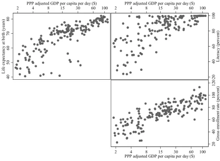
inception in 1990. The first report (“Concept and Measurement of Human Development”) specified three aspects of the quality of life to be enhanced by development: longevity, knowledge and ‘command over resources to enjoy a decent standard of living’. (Human Development Report, 1990). In practise, longevity is measured by life expectancy at birth; knowledge by the literacy rate, while purchasing power adjusted real GDP per capita is used as a stand-in for ‘command over resources’.

Anand and Sen (2000) note that the use of ‘command over resources’, and the income measure used as its stand-in (proxy), is meant to capture other basic capabilities not already included in the measures of longevity and education. However, they also stress the importance of including a measure of income, per se, in the HDI:

“Having an income is not, of course, comparable with being educated or living long, which are valued for their own sake. Having an income-related control over purchasable commodities can scarcely be intrinsically valuable. Nevertheless, in an indirect way – both as a proxy and as a causal antecedent – the income of a person can tell us a good deal about her ability to do things that she has reason to value. As a crucial means to a number of important ends, income has, thus, much significance even in the accounting of human development. While something is lost in terms of ‘purity’ in not sticking only to variables such as life expectancy and being educated which are valuable in themselves, a major practical gain is made in indirectly extending the coverage to take note of various capabilities that people do value intensely and which cannot be adequately reflected in figures of life expectancy and literacy.” (Anand and Sen, 2000, p. 100)

Hence, one can surely argue that even though growth of national income is not a synonym for development, it is an indicator of an essential part of the quality of human life.

In addition to its independent status as an important indicator of development, national income per capita also has a close association with other indicators of human wellbeing. This is

data from the Human Development Report 2007/2008. The Index has three components in total. The first, for longevity, is life expectancy at birth while the second, for knowledge, is a combination of the adult literacy rate and the gross enrolment rate (share of children at each level of schooling actually attending school). The third component, for “command over resources”, is GDP per capita adjusted for differences in purchasing power, here, converted into daily income to ease the understanding of the enormous differences.

40 50 60 70 80 L if e ex p ecta n cy at b ir th ( y ea rs )

2 4 8 15 30 60 100 PPP adjusted GDP per capita per day ($)

20 40 60 80 10 0 L it er acy ( p er ce n t)

2 4 8 15 30 60 100 PPP adjusted GDP per capita per day ($)

20 40 60 80 10 0 12 0 G ros s e n ro ll m ent r at e ( p er ce n t)

2 4 8 15 30 60 100 PPP adjusted GDP per capita per day ($)

FIGURE 1. The association between purchasing power adjusted GDP per capita and other components of the Human Development Index.

Data Source: Human Development Report 2007/2008, Human Development Indicators, Table 1.

FIGURE 2. The association between purchasing power adjusted GDP per capita and Gender Empowerment (GEM). The GEM index measures women’s economic participation and decision making, political participation and power over economic resources. Larger values mean greater empowerment. See the data source for explanation of the construction of the index.

Data Source: Human Development Report 2007/2008, Human Development Indicators, Table 1 and Table 29.

In a broader perspective, per capita GDP is correlated with essentially any indicator of the various dimensions of development that has been put forward. As another example, Figure 2 illustrates the strong association between per capita GDP and the ‘Gender Empowerment Measure’ calculated in HDR 2007/2008 revealing another stylized fact; gender equality is generally increasing with rising national income.

The strong correlation between per capita GDP and other development indicators is often used as an argument in favour of looking (only) at GDP and its growth rate. Interestingly, Anand and Sen (2000) turns this argument on its head by asking why one should not simply look at life expectancy or literacy instead of GDP. After all, life expectancy and literacy are direct measures of human wellbeing whereas GDP per capita is only an indirect measure. As the three variables are highly correlated, looking at GDP per capita may not add much information. This is a reasonable argument. The problem is however that while economists have a well-established tool box for analysing the growth process, the same cannot be said for other aspects of human

.2

.4

.6

.8

1

G

ende

r Em

pove

rm

en

t

M

ea

sure

2 4 8 15 30 60 100

wellbeing. As Robert Lucas Jr. noted awhile ago, after reviewing the basic theoretical framework that economists’ often use to study the development process:

“It seems universally agreed that the model I have just reviewed is not a theory of economic development. Indeed, I suppose this is why we think of “growth” and “development” as distinct fields, with growth theory defined as those aspects of economic growth we have some understanding of, and development defined as those we don’t.” (Lucas, 1988, p. 13).

Hence, when economists are faced with a choice between analysing economic growth and, say, life expectancy, they almost inevitably opt for analysing growth because the profession has developed a rich framework for this kind of analysis. In addition, as documented above, rising income levels do seem to be narrowly connected to more direct measures of development.7

2.2. Should the focus rather be on poverty alleviation?

Turning to the question if we should focus on poverty instead of average income (GDP per capita) in aid effectiveness analyses, it is obvious that the focus of many foreign aid initiatives is that of poverty alleviation. Further, the first millennium development goal is to “halve, between 1990 and 2015, the proportion of people whose income is less than $1 a day” (www.un.org/millennium-goals/). Hence, it may seem more relevant to focus directly on measures of poverty rather than on growth in average income. Indeed, from this (policy) perspective the critique of studies that focus on growth in GDP per capita has merit.

At the same time, one may observe that a strong focus on within country income inequality, in the context of poor countries, represents an example of an inability to “see the forest for the trees”. Consider Figure 3, which shows purchasing power adjusted GDP per capita per day for 24 of the poorest countries in the world. As is apparent, most of these countries are located in Sub-Saharan Africa. Moreover, measured on a daily basis it is clear that many of the poorest countries are hovering around the two dollar a day threshold.

7 _{In some dimensions, however, there is debate as to whether affluence brings development. An example is democracy. The} correlation between income and democratic right is strong and positive. But while there is a long tradition, going back to Lipset (1959) of believing economic prosperity also brings political reforms, this remains an area of controversy. In the cases discussed above (e.g., gender empowerment) there are well developed theories to suggest growth lead to

Chad Tajikistan Congo Mozambique Kenya

Central African Republic Burkina Faso

Rwanda Benin Nigeria Eritrea Ethiopia Mali Myanmar Zambia Yemen Madagascar Guinea-Bissau Sierra Leone Niger Tanzania

Congo (Dem. Rep.) Burundi

Malawi

0 1 2 3 4

PPP$ GDP per capita per day

FIGURE 3. Purchasing power adjusted GDP per capita per day in 24 of the poorest countries. Data Source: Human Development Report 2007/2008.

One way of thinking about these numbers is as the daily living standards of the peoples of, say, Sierra Leone in the absence of any income inequality within the country. Hence, if we were to (as a mental experiment) even out all difference in living standards within Sierra Leone, every person in the country would end up around the 2 dollar per day subsistence boundary. The poor living conditions in Sierra Leone are therefore not simply a consequence of an unequal distribution of income. If poverty is to be reduced in Sierra Leone there is only one way in which this is

feasible: by fostering growth in average income. A very similar point can be made in the context of the other countries in the figure.

This is not to say that growth in average income inevitably will improve the living standards of the poorest people within the poorest countries. But what we have to face up to is the simple realization that economic growth is a necessary condition for lasting reductions in poverty, whichever way we choose to measure the latter. It is not possible to eliminate poverty in the poorest places around the world unless growth in GDP per capita is (re-)vitalized.

Consequently, it is natural to examine whether indeed foreign aid has been able to do so.

3. The basic empirical approach to assessing aid effectiveness: Regression analysis

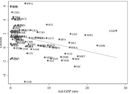
The most basic way of analyzing the association between two variables of interest is by plotting them against each other in a so-called cross-plot. Hence, as a point of departure, Figure 4 plots data on aid and growth.8 _{More specifically, Figure 4 depicts the average, percentage, ratio of aid}

to GDP from 1970 to 2000 and the average annual growth rate of GDP per capita during the same period, for 78 countries. The average annual growth rate in GDP per capita for each country is calculated as 100*[(y2000/ y1970)1/30-1] where y is GDP per capita and the subscript

indicate the year. The aid to GDP ratio is the average of the annual ratios from 1971 to 2000.

A reasonable question is why one would focus on 30 year averages, rather than averages over shorter periods of time. The answer is that the long-run average tends to “iron out” short run fluctuations in growth and aid; in the short run (say at a yearly frequency) the data on aid and growth can be quite far from the long-run trend because random events, such as weather conditions for agricultural production, are influential in a given year. The impact of variation in rainfall and other short-run fluctuations will be smoothed out when we use averages over several years. Nevertheless, it is worth pointing out that there is no objective criterion that inevitably recommends taking averages over three or four decades; shorter averages (down to say 4 or 5 years) may be sufficient to expose long-run patterns. Still, for present purposes the 30 year average will do; cross plots of the average aid-to-GDP ratio and average annual growth rate in GDP per capita always tend to look like Figure 4 regardless of the choice of base period and the length of the average involved.

Since the early 1970s, plots like Figure 4 have appeared in numerous scholarly books, journal articles and government reports analyzing aid effectiveness. There are several things one may take away from the figure. First, one may note that there is a lot of variation in terms of how much aid various countries received during the 30 year period. At one end of the spectrum we find a country like Guinea-Bissau (GNB) where foreign aid accounted for nearly 30 percent of GDP, on average. Meanwhile, in Nigeria (NGA)—to name another African country—aid accounted for less than half a percent of GDP on average. For most countries aid constitutes a fairly low fraction of their GDP. The median level of aid is just below 3 percent.9 _{To put the}

latter number into perspective one may observe that the contribution to GDP from agriculture in Denmark accounted for about 3 percent in 2000. Hence, for the “typical” aid receiving nation aid is just about as important, in accounting for GDP, as the production of agricultural foods is, in a rich place like Denmark. As some of the 78 countries received quite high aid

8 _{The data is tabulated in Annex 4.}

inflows during the period, the mean aid-to-GDP ratio is somewhat higher than the median, at 5.5 percent.

Second, from the figure we also learn that most of the 78 countries became richer during the 30 year period; the median growth rate in the sample is just below 1.4 percent. Still, this rate does fall short of the average growth rate for most rich countries like Denmark where the average growth rate was around 2 percent during the same period. Hence, the relative income difference between the typical aid recipient in the figure, and the richest places on earth, tended to grow from 1970 to 2000. Moving away from the median we may observe that the absolute level of income per capita actually fell from 1970 to 2000 in 17 of the countries in the sample.

DZA ARG BGD BEN BOL BWA BRA BFA BDI CMR TCD CHL CHN COL ZAR COG CRI CIV CYP DOM ECU EGY SLV _ETH FJI GAB GMB GHA GTM GNB GUY HTI HND HUN IND IDN IRN ISR JAM KEN KOR LSO MDG MWI MYS MLI MRT MUS MEX MAR NAM NIC NER NGA PAK PAN PNG PRY PER PHL ROM RWA SEN SLE SGP ZAF LKA SYR THA TGO TTO TUN TUR UGA URY VEN ZMB ZWE -4 -2 0 2 4 6 Gr o w th

0 10 20 30

Aid-GDP ratio

FIGURE 4. The association between the aid-to-GDP ratio 1970-2000 average, and average growth in GDP per capita (PPP) 1970-2000. See the text for explanations of the calculations.

Notes: The line in the figure is a simple regression line estimated by ordinary least squares (OLS). Individual countries are identified by a three-letter ISO code which is unique. See Annex 4 for country codes and country names.

Data Source: Rajan and Subramanian (2008).

receive more foreign aid are on average growing more slowly. However intuitive, this “visual inspection approach” has its shortcomings and sometimes the approach does not answer the questions we have in mind. For starters, it is hard to tell if the association, in a meaningful statistical sense, is systematically negative or not.

Regression analysis is a statistical technique that allows a resolution of the latter problem in the sense that it allows us to look at the “strength” of the apparent negative association. For instance, employing regression analysis we can determine how to ‘best’ draw a straight line through the observations in Figure 4. This exercise amounts to specifying a linear relationship between aid and growth. The linear relationship is expressed mathematically as

,

Growth= + ⋅a b Aid

where “b” is the slope of the line and “a” is the growth rate when no aid is given to a country. Subsequently, one may ask whether the slope of the line is positive, negative or zero, and how much confidence we should have in the association being systematic.

The regression describing the linear relationship between aid and economic growth is depicted in Figure 4. Statistically speaking the linear association is significant, which means it can be thought of as a reasonably strong association and not just a random coincidence. The statistical confidence we have in this result is high. In fact, the association is so strong that with 99% probability we reject the hypothesis that the two variables are unrelated. Hence, there is a statistically strong negative association between the development in living standards and aid disbursements, measured as a fraction of the recipient countries’ GDP.

The economic strength (as opposed to the statistical strength) of the association can also be gauged invoking the regression analysis, since we determine the slope of the line. In the present case, the slope, b, is -0.12. It is important to understand what this means.

Suppose we are observing two countries, A and B, and that the only knowledge we have about the two countries is that A receives 1 percentage point more aid than B along with the slope estimate, b = -0.12. Suppose next that we are asked what the expected growth difference is for these two countries. The answer is that we expect B to grow at a rate that is 0.12 percentage points higher than A. Naturally, this amounts to be taking the slope estimate (the numerical size of b) very seriously. That is, we need to assume the line in Figure 4 is an adequate description of A and B. Looking at the figure we know this may be problematic; some countries are far from the straight line. Still, as long as the only information we have pertains to aid flows, this is our best prediction.

Notice that the above statement does not involve words like “affects”, “leading to”, or “explaining”. In the most basic form, regression analysis does not allow us to say what created the link between aid and growth. This fact is crucial for understanding most of the aid effectiveness debate and this is why the next section discusses this issue in detail, and the

4. The cause and effect problem

This section falls in four subsections.10 _{To begin, we briefly explain why it is important to move}

beyond simple scatter plots like Figure 4 when looking at the association between two variables such as aid and economic growth. This takes us from simple regression to multiple regression analysis in order to deal with an issue called “omitted variable bias” in the econometric

literature.

Subsequently, we lay out the tricky problem associated with interpreting regression coefficients, such as those recovered through simple and multiple regression analysis. Specifically, we discuss the problem of bi-directional causality, which arises when the amount of aid disbursed to

countries has an impact on their growth rate and, at the same time, the growth rate affect the amount of aid a country receives. Bi-directional causality leads to the so-called “identification problem” in econometrics.

It is sometimes argued that the problem of bi-directional causality is more apparent than real in the context of aid effectiveness research.11 _{Therefore, we next explain exactly why this problem}

is something serious aid effectiveness research needs to deal with.

Finally, against this background, we lay out one approach econometricians have developed in order to deal with the identification problem: instrumental variable estimation.

4.1. Simple and multiple regression analysis

When looking at patterns in the data, like the one depicted in Figure 4, it is natural to wonder about its interpretation. Some analysts quickly jump to the conclusion that it reflects a casual

relationship: a high aid-to-GDP ratio causes low growth. If this is the true state of affairs there is good reason to seriously reconsider aid giving. However, there are several other reasons why a negative association between growth and aid could arise in the data.

For starters, it is possible that some other intervening variable could account for the association. To see how this works, suppose for a moment that aid does not affect growth, and that growth does not affect aid. Hence, there is no causal relationship between aid and growth. Next, imagine donor agencies have agreed to focus the lion’s share of all aid efforts on Sub-Saharan Africa (SSA). Not, suppose, because SSA is a poor region but simply because of its (strategic,

10 _{Good formal introductions to the statistical issues dealt with in the present section are given in most introductory} econometric text-books. Two popular books are Wooldridge (2008) and Stock and Watson (2007). The introductory textbooks require, however, an understanding of probability theory and statistics at, at least, a high school level. A good introduction to probability and statistics, in Danish, is given in Malchow-Møller and Würtz (2003).

say) location. Moreover, consider the possibility that growth in GDP per capita just happens to be lower in countries located in SSA compared to other developing countries. If both

propositions are true, aid and growth will be negatively related even though aid and growth are actually not causally related to one another. The association is accounted for by the interrelationship between geographical location (SSA), aid donations, and growth.

Non-SSA countries

SSA countries

Gr

o

w

th

Aid-GDP ratio

FIGURE 5. Aid and growth with geographical location as an intervening factor.

Note: The scatter plot depicts hypothetical data in which there is no direct association between aid and growth. African countries have high aid-to-GDP ratios and low growth while non-African (developing) countries have low aid-to-GDP ratios and high growth..

Figure 5 illustrates the point. If countries in Sub-Saharan Africa receive larger aid flows (relative to GDP) and at the same time have lower growth rates than countries in other continents then there is a strong tendency for countries outside Sub-Saharan Africa to cluster in the North-West corner (low aid, high growth) while Sub-Saharan African countries cluster in the South-East corner (high aid, low growth), resulting in a negative association between aid and growth when we look at all countries in the figure.

aid. As a guiding principle one should include all factors that may have an impact on both economic growth and the allocation of aid when we use regression analysis to assess the impact of aid on growth. At the same time our regression models must be kept reasonably simple if we are to learn anything from them. Hence, almost inevitably, certain determinants of growth will have to be ignored in the analysis. The problem is choosing which to ignore. Since perceived aid effectiveness will be affected by this choice, as we have just seen, it is naturally a contested issue. Indeed, it represents one explanation for the abundance of aid effectiveness studies in existence.

g= a+b*aid + x

aid = c+d*g+ z

Aid

Growth

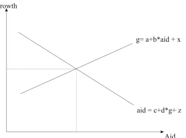
FIGURE 6. Aid and growth determined simultaneously by an aid effectiveness rule and an aid allocation rule: “bi-directional causality”.

4.2. Two rules colliding: The identification problem

Interestingly, though, the biggest problem in evaluating aid effectiveness, by way of regression analysis, arises because politician’s direct aid flows to countries where the resources are

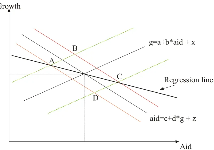
Consider Figure 6, which illustrates a possible way to think about the relationships between aid and growth in a country. The figure contains two lines—indicating two ‘rules’. On the one hand, we may hypothesize that more foreign aid increases the growth rate of GDP; this is captured by the upward sloping line that we will refer to as “the aid effectiveness rule”:

Growth= + ⋅a b Aid+x.

Notice that we allow growth to be affected by other factors beyond aid. These growth drivers are collected in the variable ‘x’, which determines the location of the line in Figure 6. For

example, we would expect x to be low for a country in Sub-Saharan Africa, while it is high for a non-SSA country. Furthermore, one may imagine that when, say, the level of education raises the variable x increases and the line shifts upwards yielding faster growth.

The slope of the line, b, reflects the impact of aid on growth. Hence, if we wish to learn about “the effectiveness of aid” this is the slope one would like to estimate or identify. In Figure 6 we

assume aid increases growth. This is certainly not the impression one is left with after studying Figure 4. Nevertheless, the present illustration will still lead to a “picture” akin to Figure 4 as will be seen.

The other line in Figure 6 captures the aid allocation policy by which a country receives less aid from the donors when it becomes richer. We call this line “the aid allocation rule”:

Aid = + ⋅c d Growth+z.

Aid allocation is also affected by other things than growth; these aid attractors are collected in the variable ‘z’. An example could be child mortality: higher child mortality translates into a higher value for z, which shifts the line upwards, resulting in higher aid levels for all possible growth rates. The slope of the line, d, reflects the impact of growth on the amount of aid a country receives.

Taken together the two lines provide an interpretation of how aid and growth is determined in a particular country, during a particular period. Specifically, the actual growth rate and amount of aid received is found as the intersection between the two lines. If the level of aid and the growth rate are determined by these two rules in every aid receiving country this will have profound impact on the interpretation of the data depicted in Figure 4. To see how, we consider some examples.

First of all, we fix the parameters of the aid effectiveness rule and the aid allocation rule. Specifically, we let the two constant terms, a and c, be equal to zero while b is 0.1 and d is -10. Then the rules become

0.1 10

= ⋅ + = − ⋅ +

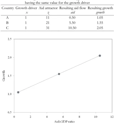
Based on the two equations, ‘observations’ for aid and growth are completely determined by the growth driver, x, and the aid attractor, z. In Table 1 we show hypothetical outcomes for three countries, A, B and C for which the growth driver is the same while the aid attractor differs across countries. This means that the countries have exactly the same aid allocation rule while the location of the aid effectiveness rule varies.

Table 1: Aid and growth outcomes for three hypothetical countries having the same value for the growth driver

Country Growth driver

x

Aid attractor

z

Resulting aid flow

aid

Resulting growth

growth

A 1 11 0.50 1.05

B 1 21 5.50 1.55

C 1 31 10.50 2.05

FIGURE 7. An example of an observed association between aid and growth when the aid allocation rule differs across countries while the aid effectiveness rule is the same.

parameter, b. In fact, we are actually tracing out the common aid effectiveness rule by combining the data points.

In Table 2 we consider another set of countries, A’, B’ and C’. The three countries have exactly the same aid effectiveness and aid allocation rules as before, but they differ in the values of their growth drivers and aid attractors. The three new countries share the same value of the aid attractor while the values of the growth drivers differ. Thereby the countries have a common location of the aid allocation rule while the location of the aid effectiveness rules varies.

Table 2: Aid and growth outcomes for three hypothetical countries having the same value of the aid attractor

Country Growth driver

x

Aid attractor

z

Resulting aid flow

aid

Resulting growth

growth

A' 0 21 10.50 1.05

B' 1 21 5.50 1.55

C' 2 21 0.50 2.05

FIGURE 8.An example of an observed association between aid and growth when the aid effectiveness rule differs across countries while the aid allocation rule is the same.

combining regression line is -0.1 in Figure 8 compared to 0.1 in Figure 7. The slope we observe in Figure 8 is actually the inverse of the slope of the aid allocation rule: 1/d = 1/(-10) = -0.1. The reason is that in Figure 8 the aid effectiveness rule varies while the aid allocation rule is common for the three countries and what we see is the aid allocation rule (turn the page counter clock wise) not the aid effectiveness rule.

g=a+b*aid + x

aid=c+d*g + z

Aid Growth

A

B

C

D

Regression line

FIGURE 9B. The observed association between aid and growth when both the aid effectiveness rule and the aid allocation rule vary across countries.

Moving a little closer to the real world we know that every country will have their own value of both the growth drivers, x, and the aid attractors, z. So, the actual observations will be scattered around as in Figure 4. To illustrate, in Figure 9A we plot observations for the nine hypothetical countries that can be observed when we combine the three values of x (0, 1, 2) and the three values of z (11, 21, 31) from tables 1 and 2. The relationship between aid and growth will be positive or negative, depending on your choice of angle. However, the regression line in Figure 9A has a slope of zero, indicating no systematic relationship between aid and growth.

Figure 9B illustrates the general problem of having two rules generating the actual data. We have a lot of different, parallel, aid effectiveness rules (one for each country in a particular period) and just as many different, parallel, aid allocation rules. For the illustration we assume there is a maximal and a minimal value of the growth drivers, x, leading to a maximal and a minimal aid effectiveness line. Likewise we assume a maximal and a minimal level for the aid attractor, z, giving a maximal and a minimal aid allocation line. Since each data point, according to this simple model, is thought to reflect a point of intersection between the two rules, all data observations would appear in the area ABCD. If we use ordinary least squares regression to assess the link between aid and growth, the resulting line would tend to go through the points A and C. Crucially, observe that the slope of this line will not be equal to either the aid

aid allocation rule. The opposite is also true; if the variation in the aid allocation rule is larger than the variation in the effectiveness rule we get closer to the aid effectiveness rule.12

In essence, the examples show that if our data is the outcome of two rules then just observing the data points we have no way of knowing if we are estimating one rule or the other.13 _The

bottom line is that a regression coefficient cannot be interpreted as reflecting a causal impact of aid on growth (or growth on aid, for that matter). This is what economists’ call “the

identification problem”.

Figure 10 summarizes the possible interpretation of (any kind of) correlation between foreign aid and economic growth. In the example from Section 4.2 “geography” is an “intervening variable”, whereas the bi-directional link between aid and growth, illustrated by the two

separate lines in Figures 6-9, is captured by the arrows connecting the growth and aid “boxes” in the figure.¨

FOREIGN AID ECONOMIC GROWTH INTERVENING

VARIABLES

FIGURE 10. Possible reasons for a correlation between foreign aid flows and economic growth.

4.3. Is it really a problem?

At times one may come across research where the identification issue is not recognized, or, is “winked away”. In the best of cases there is an argument in favour of ignoring the problem. If so the argument is that the notion of “bi-directional” causality, leading to the identification problem, is a fallacy. After all, there is little (if any) evidence that aid is given to the countries that grow at the slowest speed. To be sure, there is amble evidence that aid is given

predominantly to the poorest countries. Consequently, if the analysis focused on the link between

12 _{Technically speaking the two curves could also be shifting around due to statistical disturbances, which affect the} individual curves. Hence, these shifts need not reflect differences in other determinants of growth and aid.

aid and the level of income the identification issue would be very real. However, the argument goes, there is likely no reverse causality problem between aid and growth of income. In other words, the aid allocation rule in Figure 6 does not exist. If true, all a researcher needs to do is to include the level of income per capita as an intervening factor in the growth regression and the problem is solved. Unfortunately, this reasoning is flawed.

Understanding this point is critical because we, in effect, dismiss a large part of about 40 years of scholarly research on the topic. Most aid effectiveness analyses before 1995 did not take bi-directional causality into account (see Hansen and Tarp, 2000). Therefore, to prove the point, we proceed in small steps.

To simplify the exposition assume aid has no causal impact on economic growth. That is, assume the slope, b, in the aid effectiveness rule, that we are trying to find, is zero.

Next, consider two countries that are identical with respect to GDP per capita and aid flows in 1970. That is, they are of equal size, equally rich and they receive the same amount of aid. Imagine (for now) the two countries receive a constant flow of aid, measured in real US dollar per capita, each year from 1970 to 2000. Now , let’s assume one country (A, say) is hampered by problems leading to zero growth in GDP per capita, on average from 1970 to 2000 while the other country (B) is doing better, experiencing an average growth in GDP per capita of two percent a year during the same period of time.

While we thus know that the two countries receive exactly the same amount of aid per capita, and that this translates into the same share of aid-to-GDP in 1970, it is also clear that they will not have the same aid-to-GDP ratio in 2000 (or in any other year after 1970 for that matter). If both countries have an aid-to-GDP ratio of five percent in 1970, then country A will

experience an average ratio of exactly five percent over the period, as the aid flows are constant and the average annual growth rate is zero. However, the annual aid-to-GDP ratio will not be constant in country B; it will be declining because the aid flow is constant while GDP per capita is increasing. A few calculations show that when the average growth rate is two percent a year, the average aid-to-GDP ratio, from 1970 to 2000, is roughly four percent in country B. Hence, the fastest growing country will have the lowest observed aid-to-GDP ratio. Yet, in this simple example the aid-to-GDP ratio is low precisely because the country is growing rapidly; not because aid is harmful.

association between aid (to GDP) and growth.14 _{Note that the larger the differences in the}

growth rates, the steeper the slope of this allocation rule.

But aid flows are clearly not constant over time. In fact, it is a widespread finding that, once intervening factors are controlled for, aid per capita decreases with the level of GDP per capita. The question is how this will impact on the aid-growth association that we observe in the data. Again, we simplify to illustrate the effect in a transparent way. So, imagine the donors make their aid allocation decisions collectively once every decade, starting in 1970. Further, assume the donors follow an allocation rule saying that when GDP per capita is increased by one percent in a country, aid per capita is cut by one percent.

Now, reconsider countries A and B. They have the same aid flows per capita in the 1970s because they have the same GDP per capita in 1970. The initial aid-to-GDP ratio is five percent. But due to the differing growth rates—zero percent in country A and two percent in B—they will not receive the same aid flows from 1980 onwards. In fact, in 1980 country B is more than 20 percent richer than country A. (22 percent to be precise). This means that in the 1980s aid per capita will be cut back by 20 percent in country B. Country A, by contrast, will receive the same amount of aid since its income per capita level is the same. Note, however, that as country B is both richer and receives less aid per capita in 1980, the aid-to-GDP share is now more than 40 percent lower in country B compared to country A. This pattern is amplified after 1990 since country B is now almost 50 percent richer than country A (which still is at the 1970 level of both countries), implying aid flows to B are cut by 50 percent compared to the 1970 level. In 2000 country B is about 80 percent richer than country A because of the difference in the average growth rates of two percent per year. When we calculate the average

aid-to-GDP share over the 30 years, 1970 – 2000, country A will have the same share as in the case of constant disbursements: five percent. In country B we have three decades of (step-wise) declining aid flows coupled with persistent growth in GDP per capita; the average aid-to-GDP ratio is just above three percent for country B; lower than the four percent average calculated with constant aid flows.

The general point to take away from this illustration is that the negative association between the average aid-to-GDP ratio and growth becomes more pronounced when donors are active in periodic reallocation of aid guided by the level of GDP per capita. Without reallocation of aid funds the fast growing country (B) obtained an average aid-to-GDP ratio of four percent; with reallocation the ratio shrinks to about three percent.

Aid allocation is of course not a decision made at collective meetings for all donors once every decade, but a mix of decisions made by individual donors at varying intervals. This will,

however, only tend to strengthen our result, which establishes a strong causal influence of growth on aid.15

The identification problem, as discussed in Section 4.2, is therefore very real. Accordingly, to elicit information about the impact of aid on growth we need to deal with it; it cannot

reasonably be winked away.

4.4. A possible solution to the cause and effect problem

Ideally one can imagine a simple fix to the identification problem; randomized trials. Such experiments, which are akin to the testing procedures used when new drugs are evaluated, have many supporters at the project level.16 _{Evaluating aid at the country level we need to imagine}

random helicopter drops of aid money across the globe. In this universe any correlation between aid and economic growth could not be ascribed to correlations with other variables (the intervening variables problem), nor reverse causality.

Naturally, this is not really an option (politically, at least): few people would find it reasonable for aid to be disbursed to middle income countries, like Argentina, rather than the most in need, just to elicit information about whether it works or not. And this could be the outcome of the random trial. Hence, absent a good experiment economists have to rely on statistical methods to try to resolve the problem at hand. A way forward is what econometricians call

“instrumental variables estimation”.

To understand the basic logic of the approach, consider Figure 11, which is a slightly

augmented version of Figure 10: the new feature being the box labelled “instrument”. What this box is supposed to encompass is a factor which affects aid disbursements. Yet, it is not just any determinant of aid flows. Notice that the box involving “instrument” is not connected to

any other box, aside from aid. Hence the instrument does not affect growth (above its impact via aid), it is independent of other factors (intervening variables) that explain growth, and it is not itself explained by growth.

15 _{For a mathematical proof of this point, see Annex 2. A proof of the reverse causality result in a much more general setting} is given in Dalgaard, Hansen and Tarp (2004).

FOREIGN AID ECONOMIC GROWTH INTERVENING

VARIABLES INSTRUMENT

FIGURE 11. Teasing out the causal effect from aid to growth using instruments.

To see how this works, suppose for a moment that we have located such a variable. To fix ideas let us call it “size”, measuring the size of countries by, say, the population size. We can now perform the following “statistical experiment”. First we figure out how much of the cross-country differences in aid levels we can explain with the cross-country size variable. That is, we quantify the strength of the arrow between the instrument (country size) and aid in Figure 11. Second, we take the amount of aid that size—and only size—can motivate in each country in the world, and look at the association with observed growth rates in these countries. If a significant association prevails we say that this is because aid affects growth.

Why must this be the case? If there is a link between size-generated-aid and growth rates we know this correlation cannot be explained away by reverse causality: growth in GDP per capita does not explain the size of a country (cf. the absence of any arrow from growth to

“instrument” in Figure 11). Hence, reverse causality is ruled out. Next, the association cannot be explained away by intervening variables either, since country size is not related to these variables (cf. the absence of any link between “instrument” and intervening variables in Figure 11). Finally, country size does not explain growth directly (cf. the absence of any arrow from “instrument” to growth in Figure 11). If all of this is true, the only interpretation of the

g= a+b*aid + x

aid = c+d*g+ z

Aid

Growth

Δ

z

Z

FIGURE 12. The Geometry of instrumental variable estimation. Notes: In the text we refer to “z” as country size. The bottom panel shows the link between country size (z) and aid

allocation. The top panel concerns the link between aid and growth.

get variation in the allocation rule which is independent of the effectiveness rule—such that the allocation rule moves while the effectiveness rule is fixed. This is exactly the situation in which the data will trace out the aid effectiveness rule as depicted in Figure 7. Consequently, we have thereby identified the impact of aid on growth statistically.17

Despite the apparent simplicity, the major problem with this procedure should be clear: it is hard to find a determinant of aid flows which fulfils the requirements for it to act as an instrument for aid. To see how the experiment could fail, consider the following line of

reasoning. Suppose smaller countries do in fact receive more aid per capita and as a fraction of GDP per capita, as assumed above. This makes population size a candidate for being an instrument. However, suppose the population size affects growth directly. That is, imagine population size has an impact on growth above and beyond its potential impact via aid. In particular, imagine “size is good for growth”.18 _{If so, we are back to square one. A negative}

association between aid (as explained by country size) and growth may now be taken to imply either a negative impact of aid flows on growth, or, that big countries are growing faster due to their size, and simultaneously receive less aid. In terms of Figure 12, the problem can be seen as that of the instrument shifting both lines around, rather than just the aid allocation rule. In this case the procedure does not trace out the slope of the aid efficiency rule. We have thus not solved the problem of identifying the impact of aid on growth.19

These difficulties have been a main impetus for the aid effectiveness debate over the last decade or so. We take up another reason for the debate later in this study. But first, in the next section, we provide an illustration of how estimates change, when we try to deal with omitted variable bias and, in particular, the identification problem.

17 _{A mathematical demonstration of this point is found in Annex 3.}

18 _{There are several reasons why this could be the case. For instance, in larger countries there may be greater scope for} division of labor which stimulates growth; an idea that goes back to Adam Smith’s “Wealth of Nations’’.

19

5. An illustration of the regression approach

If indeed there is a severe identification problem to deal with we should be able to illustrate the consequences of taking it into account using actual data. This section provides such an

illustration. The data we use are from a recent study by Rajan and Subramanian (2008) and we begin the illustration by presenting the regression line in Figure 4. Expressed as an equation this line reads as

1.92 0.12

(0.31) (0.04)

= − ⋅

Growth Aid

The two parameters of the equation are estimated using ordinary least squares. Below the parameter estimates we show the standard errors of the estimates in parentheses. The standard errors give an indication of the precision of our estimates and, thereby, of the confidence we can have in the specific values. In general, small standard errors indicate precise parameter estimates and, as a rule of thumb, we say that if a parameter divided by its standard error is above 2, in absolute terms, then the parameter is statistically significant. This means that we consider the parameter to be different from zero whereby the variables we study are considered to be systematically related. In the equation above the slope coefficient divided by its standard error is -3, leading us to the conclusion of Section 3, that the negative association between aid and growth is highly significant.

-4

-2

0

2

4

6

Gr

o

w

th

0 10 20 30

Aid-GDP ratio

Sub-Saharan African countries Other countries

FIGURE 13. The association between the aid-to-GDP ratio and average growth in GDP per capita (PPP) 1970-2000. Highlighting countries in Sub-Saharan Africa (circles) and other countries (diamonds).

Data Source: Rajan and Subramanian (2008).

Average of all 78 countries

Average of 32 countries in Sub-Saharan Africa

Average of 46 countries outside

Sub-Saharan Africa

Growth 1.2 0.2 1.9

Aid-to-GDP ratio 5.5 10.0 2.4

TABLE 3. Average growth rates and Aid-to-GDP shares inside and outside Sub-Saharan Africa

This assertion can be investigated using multiple regression analysis. We simply augment the regression above with a variable that takes the value 1 for all countries in Sub-Saharan Africa and the value 0 for other countries. (The variable is denoted SSAfrica). The resulting regression is

2.10 0.06 1.22

(0.27) (0.06) (0.68)

= − ⋅ − ⋅

Growth Aid SSAfrica

Geographical location appears to explain quite a bit of the negative association between aid and growth. When we include the information about location in the regression the slope of the line is halved, from -0.12 to -0.06, and the coefficient divided by its standard error is now only -1, which is clearly less than 2 in absolute value, leading us to conclude that—‘conditional on geographical location’—the association is not statistically significant.20

The new result can be illustrated in two ways. A very common way is to show that geographical location is actually moving the aid-growth line, as illustrated by the inclusion of ‘x’ in the figures in Section 4. Figure 14 shows how we can draw two parallel fitted lines in the cross-plot, one for countries in Sub-Saharan Africa and one for other countries. As the lines are parallel the slopes are equal (-0.06). The intercept for ‘other countries’ is 2.10 while the intercept for the Sub-Saharan African countries is 0.88 (= 2.10-1.22).

-4

-2

0

2

4

6

Gr

o

w

th

0 10 20 30

Aid-GDP ratio

Sub-Saharan African countries Other countries

Fitted line for SSA countries Fitted line for Other countries

FIGURE 14. The association between the aid-to-GDP ratio and average growth in GDP per capita (PPP) 1970-2000. With regression lines for Sub-Saharan African countries and other countries.

Data Source: Rajan and Subramanian (2008).

BEN BWA BFA BDI CMR TCD ZAR COG CIV ETH GAB GMB GHA GNB KEN LSO MDG MWI MLI MRT MUS NAM NER NGA RWA SEN SLE ZAF TGO UGA ZMB ZWE DZA ARG BGD BOL BRACHL CHN COL CRI CYP DOM ECU EGY SLV FJI GTM GUY HTI HND HUN IND IDN IRN ISR JAM KOR MYS MEX MAR NIC PAK PAN PNG PRY PER PHL ROM SGP LKA SYR THA TTO TUN TUR URY VEN -5 0 5 Gr o w th | S-A fr ic a

-10 0 10 20

Aid-GDP ratio | S-Africa

FIGURE 15. The association between the aid-to-GDP ratio and average growth in GDP per capita (PPP) 1970-2000 when group averages are subtracted.

Data Source: Rajan and Subramanian (2008).

Based on the data in Figure 15 we can again draw the best fit line to illustrate the linear association between aid and growth, which is now conditional on geographical location. The slope of the line in Figure 15 is -0.06—exactly the slope in the regression equation above. The intercept is zero by construction because we have removed the means of the two variables. The important message to take away from Figure 15 is that when we include other variables in a regression, we ‘control’ for the effect of the variables by generating new observations. The new observations are in some sense more ‘true’ than the original because they are not blurred by the intervening factors. In general, we can control for as many intervening factors we like. This can always be done by generating new observations showing the conditional association between aid and growth.

the value of GDP per capita in 1970.21 _{In total our regression has four explanatory variables}

and an intercept.

11.17 0.09 1.97 9.49 1.78

(2.31) (0.05) (0.56) (1.86) (0.29)

= − ⋅ − ⋅ + ⋅ − ⋅

Growth Aid SSAfrica Institutions GDPcap(1970)

In this regression, all factors, except for aid, have significant slopes measured by the absolute size of the slope divided by standard error. The effects of the three intervening factors are in line with economic reasoning: growth is lower in Sub-Saharan Africa, as already discussed; “good institutions” are associated with higher growth rates, and initially richer countries tend to have lower growth in the subsequent years—everything else being equal.22

The conditional association between aid and growth is again negative, with a slope of -0.09, which is nicely between the -.12 we found in the simple regression and -.06 that came out when we only condition on Sub-Saharan Africa. Variation in the estimated slope of this order of magnitude is quite common and it shows that aid flows are correlated with the other factors in the regression model. Again, we find that the coefficient divided by its standard error is less than 2 in absolute value whereby we conclude that the conditional association between aid and growth is statistically insignificant. A cross-plot of the aid and growth observations, in which variation due to geography, institutions and initial richness has been removed, is given in Figure 16. The slope of the regression line in the figure is -0.09 as reported in the regression above and the intercept is zero by construction.

We can now turn to the instrumental variable regression. Rajan and Subramanian (2008) have constructed an instrument, partly based on country size but also on other factors, that should not have a direct impact on growth.23 _{By the instrumental variable regression approach we must}

first establish the linear association between aid and the instrument and, further, we must ensure that the association is not driven by the intervening factors already included in the model. This is done via a regression, known as the first-stage regression in the econometric literature. The regression has aid as the dependent variable while the instrument and the intervening factors are the explanatory variables:

21 _{How to measure the quality of legal institutions is an area of research in itself. We use a measure which is very popular} within economics. The data is commercial and known as the international country risk guide (ICRG). See

http://www.prsgroup.com/ICRG.aspx for a description of the data and Rajan and Subramanian (2008) for a description of

the transformation of the ICRG data in the regression analysis.

22 _{The last result is known as “conditional convergence’’ in the growth literature. See Barro (1991) for a discussion and early} evidence of the phenomenon.

DZA ARG BGD BEN BOL BWA BRA BFA BDI CMR TCD CHL CHN COL ZAR COG CRI CIV CYP DOM ECU EGY SLV ETH FJI GAB GMB GHA GTM GNB GUY HTI HND HUN IND IDN IRN ISR JAM KEN KOR LSO MDG MWI MYS MLI MRT MUS MEX MAR NAM NIC NER NGA PAK PAN PNG PRY PER PHL

ROM _SEN RWA

SLE SGP ZAF LKA SYR THA TGO TTO TUN TUR UGA URY VEN ZMB ZWE -4 -2 0 2 4 G row th | othe r va ri ab le s

-10 -5 0 5 10 15

Aid-GDP ratio | other variables

FIGURE 16. The association between the aid-to-GDP ratio and average growth in GDP per capita (PPP) 1970-2000 when geography, institutions and initial GDP per capita is controlled for.

Data Source: Rajan and Subramanian (2008).

32.22 0.62 1.97 3.00 3.76

(4.95) (0.12) (1.03) (3.79) (0.76)

= + ⋅ + ⋅ − ⋅ − ⋅

Aid Instrument SSAfrica Institutions GDPcap(1970)

In the first-stage regression it is not the size of the parameters but rather the statistical

Figure 16, because the first stage regression is just a standard regression. The association is shown in the bottom part of Figure 17.

DZA ARGBGD BEN BOL BWA BRA BFA BDI CMR TCD CHL CHN COL ZAR COG CRI CIV CYP DOM ECU EGY SLV ETH FJI GAB GMB GHA GTM GNB GUY HTI HND HUN IND IDN IRN _ISR JAM KEN KOR LSO MDG MWI MYS MLI MRT MUS MEX MAR NAM NIC NER NGA PAK PAN PNG PRY PER PHL ROM_SENRWA

SLE SGP ZAF LKA SYR THA TGO TTO TUN TUR UGA URY VEN ZMB ZWE -4 -2 0 2 4 G row th | o the r v ar ia b le s

-10 -5 0 5 10 15

Filtered Aid-GDP ratio | other variables

DZA ARG BGD BEN BOL BWA BRA BFA BDI CMR TCD CHL CHN COL ZAR COG CRI CIV CYP DOM_ECU EGY SLV ETH FJI GAB GMB GHA GTM GNB GUY HTI_HND HUN IND IDN IRN ISR JAM KEN KOR LSO MDG MWI MYS MLI MRT MUS MEX MAR_NAM NIC NER NGA PAK PAN PNG PRY PER PHL ROM RWA SEN SLE SGP ZAF LKA SYR THA TGO TTO TUN TUR UGA URY VENZMB ZWE -1 0 -5 0 5 10 15 In st ru m en t

-10 -5 0 5 10 15

Aid-GDP ratio | other variables