Munich Personal RePEc Archive
Re-examining Kuznets Hypothesis: Does
Data Matter?
Jalil, Mohammad Muaz
North South University
August 2009
Online at
https://mpra.ub.uni-muenchen.de/72557/
Re-examining Kuznets Hypothesis:
Does Data Matter?
Mohammad Muaz Jalil
Student ID# 071 889553
Department of Economics
North South University
Re-examining Kuznets Hypothesis:
Does Data Matter?
Submitted By
Mohammad Muaz Jalil
Student ID# 071 889553
Thesis Supervisor:
Dr.
A.K.M Atiqur Rahman
Professor, Department of Economics
Thesis Examination Committee
Chairman
Dr. A. K. M. Atiqur Rahman
Professor, Department of Economics North South University
Members
Dr. Mohammad Ali Rashid
Professor, Department of Economics & Dean, School of Arts and Social Sciences
North South University
Dr. Amirul Islam Chowdhury
Professor, Department of Economics Dean, School of Business
North South University
Dr. Gour Gobinda Goswami
Associate Professor & Proctor, Department of Economics
A
CKNOWLEDGEMENT
I would like to extend my gratitude to several people who have made this thesis a reality.
First of all I wish to thank my thesis supervisor Dr. A. K. M. Atiqur Rahman Professor, Department of Economics, for his time, patience, support, guideline and encouragement every step of the way. Working with him was a great learning experience and I hope to utilize this in my future endeavors.
I am really grateful to my family for encouraging me to write this thesis and for their continuous concern and support.
Table of Content
I. Introduction 8
II. The Inequality Datasets 13
III. Income Inequality And Explanatory Variables 18
IV. Econometric Issues Panel Unit Root Tests 24
V. Alternative Estimation Of Inequality Relationship 28
VI. Analysis 45
VII. Conclusion 59
VIII. References 61
IX. Appendix 1 : Descriptive Statistics Inequality Dataset 65
X. Appendix 2: Fixed Effect Ar1 On Unconditional Kuznets Curve 72
List of Tables
Table 1: The distribution of inequality measures by different definitions in D & S data ... 13
Table 2: Studies on openness and inequality ... 21
Table 3: Relevant Variables and Labels ... 23
Table 4: Panel Unit Root test ... 26
Table 5: Pooled regression on annualized dataset, all countries ... 29
Table 6: Pooled regression on Average dataset ... 31
Table 7: Pooled regression on OECD dataset ... 32
Table 8: Fixed effect regression for Unconditional Kuznets curve on Annualized all countries ... 35
Table 9: Fixed effect regression for Unconditional Kuznets curve on OECD countries ... 35
Table 10: Fixed effect regression on Annualized all countries and OECD dataset ... 37
Table 11: Fixed effect regression on annualized all countries and OECD dataset with AR1 ... 40
Table 12: Arellano-Bond on annualized all countries and OECD dataset ... 43
Table 13 : Descriptive Statistics for inequality measures ... 47
Table 14: Descriptive Statistics for inequality measures ... 47
Table 15: Distribution of inequality measures by different definitions in WIID2 data ... 49
Table 16 : Descriptive Statistics for inequality measures OECD ... 51
Table 17 : Descriptive Statistics for inequality measures OECD ... 52
Table 18 : Correlation in OECD dataset ... 55
Table 19 : Correlation in Global Dataset ... 56
Table 20: Descriptive Statistics Ln Theil and Ln D &S ... 57
List of Figures
ABSTRACT
I.
Introduction
Five decades ago, Simon Kuznets (1955) expressed the important hypothesis that income inequality first increases, but after a turning point it decreases in the course of economic development. This premise, usually termed Kuznets’s hypothesis or Kuznets’s inverted-U, has been widely investigated, but the results of that research are far from well established. Kuznets’ original hypothesis relied on historical data for the first half of the nineteenth century from only three developed countries, the US, the UK and Germany, and he cautiously concluded that the data appeared to ‘justify a tentative impression of constancy in the relative distribution of income before taxes, followed by some narrowing of relative income inequality after the first world war — or earlier’1. Kuznets (1955) did not set out a formal theory of the relationship between the degree of income inequality within a country and its level of economic development; but he drew an argument.
Here is how Kuznets curve is supposed to work: in early stage of development investment opportunities for those who have money multiply, while wages are kept low due to influx of cheap labor from rural to urban areas. In Kuznets own words “An invariable accompaniment of growth in developed countries is the shift away from agriculture, a process usually referred to as industrialization and urbanization.” With industrialization concomitantly inequality increases. Hence you get in to a situation where there are many business moguls coexisting with large body of impoverish day laborers. But gradually this urbanization or rural urban migration flattens out, hence wages begin to rise. At the same time education, enhanced social and political consciousness forces government or people in power to undertake redistributive efforts. These forces combine together to reduce inequality.
As of date the hypothesis has found many supporters, to the point of being considered ‘fully confirmed’ by Oshima (1970), a ‘stylized fact’ by Ahluwalia (1976a), and an ‘economic law’ by Robinson (1976). Recent literature nonetheless has been more cautious in their conclusions. They note that the statistical significance of the income variables of the basic
Kuznet model2 tend to get eliminated with addition of other right-side variables such as education (Bourguignon and Morrison, 1990). Many studies however studies go on supporting empirically the hypothesis, as is the case of Dawson (1997), Li et al. (1998), Barro (2000), Thornton (2001), and Huang (2004). Similarly there are those who question the hypothesis, as did Adelman and Morris, (1973); Saith, (1983), Papanek and Kyn, (1986). More recently other skeptical authors have joined this group, who challenge the hypothesis, as for example Hsing and Smith (1994), Deininger and Squire (1998), or Mátyás et al. (1998) who labeled the hypothesis as a ‘myth’. So, the hypothesis remains a theme of substantial debate in development literature.
In order to rigorously test the Kuznets hypothesis it is necessary to at least use longitudinal data although panel data structure is even better. Kuznets himself, as mentioned before, used time series data for three countries to formulate his hypothesis. Since at that time panel data analysis did not exists and neither did adequate level of inequality data, it was impossible for Kuznets to go beyond his conjecture. Even thought panel data analysis has existed for quite sometime, lack of adequate data on inequality forbade its use and hence most early researchers had to employ dataset which were almost entirely cross-sectional in nature, with typically one3 observations per country. With these data, a number of studies found support for the Kuznets curve (Ahluwalia, 1976a, 1976b; Campano & Salvatore, 1988; Chenery & Syrquin, 1975; Dawson,1997; Eusufzai, 1997; Jha, 1996; Kravis, 1960; Mbaku, 1997; Papanek & Kyn, 1987; Paukert, 1973; Randolph & Lott, 1993; Tsakloglou, 1988; Bourguignon, 1994; Milanovic, 1995; Jha, 1996).
In so far as the lack of inequality data is concerned, Deininger and Squire’s effort (hereafter D&S, 1996) is monumental. D&S collected many different surveys of income inequality, and compiled those meeting certain criteria of process4 into a single “high-quality” panel, offering 693 country/year observations since 1950. Although this dataset allows for undertaking panel data analysis, but when one tries to undertake analysis with all countries
2 With inequality measure as dependent and income variable (with quadratic term) as regressor 3 Sometimes a few observations per country were also available
4 Three main criteria are that observations should be (1) drawn from a published household survey, (2) based on
included, degrees of freedom is significantly reduced and then there may not be sufficient data points. Even with this limitation, in absence of alternatives, this is now a standard reference, on which dozens of papers have been based. Deininger and Squire (1998) using their own dataset rejected the presence of the Kuznets curve for the fixed-effects case. They do find it present in the pooled case for their functional form (namely real GDP per capita and 1/(real GDP per capita)). Barro (2000) uses a different functional form (log y and its square) and finds the inverted-U shape present in both the crosssectional pooled and fixed-effects cases. Anand and Kanbur (1993) found that the functional form chosen to test the inverted-U hypothesis could have considerable impact on the ‘turning point’, of the curve, where inequality begins to decline. They also found that the U-shape is significant for some functional forms and not for others.
More recent studies have adopted a panel data approach by using the Deininger and Squire (1996) data set and have obtained different forms of the inequality-growth relationship (Ram, 1997; Barro, 2000; Forbes, 2000). However, the D & S data set has been criticized for not generating an accurate outcome since many of its observations are not consistent and comparable, even after applying “high quality filters”, and because its coverage is limited and unbalanced (Atkinson et al., 2001; Galbraith and Kum, 2002). Still other recent papers have used the Deininger and Squire (1996) dataset (updated, with more observations) and also used country-specific fixed effects. Higgins and Williamson (1999) examine the impact of openness and cohort size on inequality in addition to the Kuznets process and found that Kuznets Curve comes out of hiding when the inequality relationship is conditioned by the cohort size. Munir and Muaz (2004) used new datasets introduced by University of Texas inequality project, UTIP. The study used 24 countries purposely selected to develop a balance panel covering LDCs, developing countries and developed countries, over a time period of 37 years from 1963 to 1999. The results were negative for both level and log quadratic formed of equations that were tested for. Time series analysis was also performed on individual countries and the results were still negative.
used, conditionality imposed (independent variables), and the econometric model used. Also one of the major limitations of the studies has been comparability of the data across countries. The present study will try to address all of these issues in a systematic manner. The ultimate objective is to bring a reasonable consensus in relation to Kuznets hypothesis. In order to achieve this objective the paper will undertake the following:
1. Four different types of inequality dataset will be used as dependent variable, namely World income inequality database (WIID2), UTIP UNIDO Manufacturing Pay inequality dataset (UTIP), Estimated Household Income Inequality Data Set (EHII) and D&S, 19965.
2. Gamut of explanatory variables will be used, taken from existing literature, to see: a. The affect of such variables on the Kuznets relationship. Whether presence of
certain explanatory variables remove the significance or alters the sign of the income variables, as some research have shown.
b. The relationship that exists between inequality and such explanatory variables and to analyze the stability of such relationship. Whether such relationship varies across the types of inequality dataset used or the structure of the dataset or the econometric method employed
3. Stationarity test will be used to ascertain the correct functional form of the econometric model, whether one has to use variables in their log or level form. Anand and Kanbur (1993b) found that the functional form chosen to test the Kuznets hypothesis can have considerable impact. They found that the inverted U-shape is significant for some functional forms and not for others.
4. Analysis will be carried out on three separate dataset, namely a. Annualized global dataset of 188 countries
b. 4 years average of the global dataset c. A dataset including only OECD countries
The objective of employing these 3 types of dataset is to assess if the structure of the data itself has any impact on the Kuznet hypothesis and the relationship between inequality and the other explanatory variables. Also many studies like Higgins and Williamson (1999), Ram (1991 and 1997), Alderson and Nielsen (2002) etc, only researched on OECD countries. Hence it is worth noting whether this has any impact on the Kuznets hypothesis. 4 years average is used to reduce serial correlation and also because researchers have often suggested that inequality is likely to be a stable across time. It is worth noting whether smoothing the dataset has any impact in determining the presence or absence of Kuznets curve.
5. Various econometric methods will be used in line with current literature and as the data demands. Literature suggests that most often used models are pooled regression and fixed effect model. However some recent researchers like Galbraith and Kum (2004), Meschi and Vivarelli (2007) employ dynamic panel model, specifically Arellano and Bond GMM methodology. While earlier researches have used cross sectional data in absence of adequate panel data, since we do not face this constraint it seems inappropriate to use this method; hence this will not be included in this paper.
Although it is improbable to answer all queries but it is hoped that present study will go a long way in testing the robustness of the elusive Kuznets curve and possibly provide key reasons for existence or absence of Kuznets curve under different circumstances.
II.
The Inequality Datasets
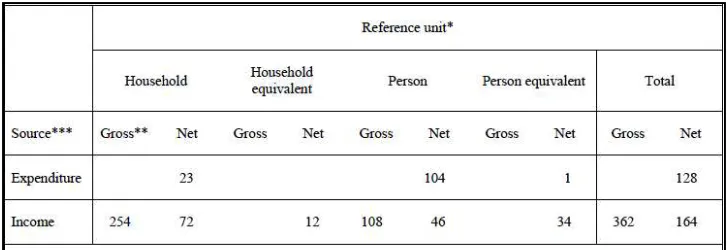
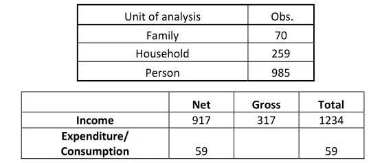
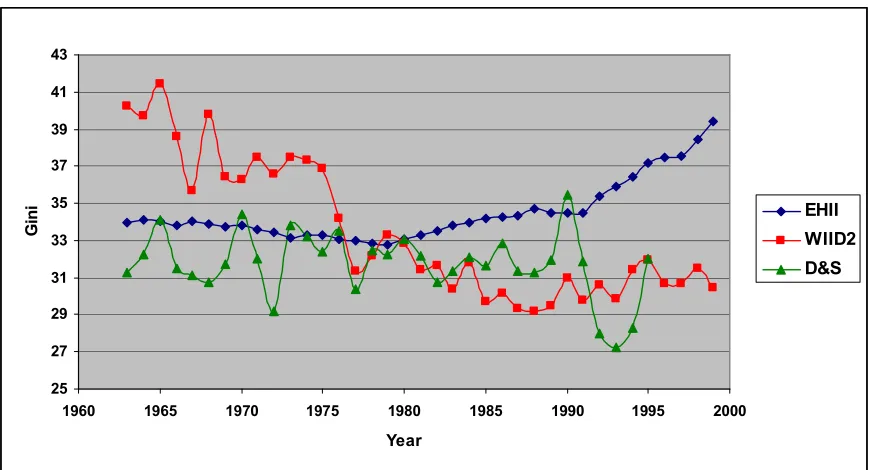
[image:14.612.133.497.496.621.2]Deininger and Squire collected many disparate surveys of income and expenditure inequality, and compiled those meeting certain criteria of process1 into a single “high-quality” panel, offering about 693 country/year observations since 1947. The database uses different sources to compute Gini coefficients, depending on the data available in each country. There are three major differences. The first is whether the unit of analysis is a household or an individual. If, as is usually the case, poor households have more members, the distribution of income at a household level will be more equal than when computed at the individual level. Therefore, one would expect to find that the Gini coefficients are greater (more unequal income distribution) in countries that report data at the individual level. The second issue is whether income data refers to income before or after tax. Provided the tax system is progressive, countries that collect data on gross (before-tax) income will probably have a higher Gini coefficient than countries that report data on net income. Finally, some countries measure the distribution of income, while others measure the distribution of expenditure, which is measured on the basis of net income. In addition, given that high income households presumably save a bigger proportion of their income than poor households, it is expected that countries that use income rather than expenditure will have higher Gini coefficients.
From the above table we see that 50% of the data in D&S is based on household estimates, gross and net inclusive. Similarly 54% of the data are based on are gross estimate, that is before tax deduction. Income based inequality measures accounts roughly 80% of the total data. Hence it is very likely that the gini measured by D&S is likely to be an overestimation of the actual underlying inequality scenario.
Despite the large number of observations, the coverage of the D&S data set remains limited and unbalanced. Serious questions have been raised as to whether the data points are in fact comparable either across countries or through time. As Atkinson and Brandolini (2001) especially argue, the D&S inequality measures are based on various income definitions, reference units and processing procedures that cannot be wholly reconciled to each other, even with “high-quality” filtering. Even within individual countries, the range of fluctuation in the D&S data is occasionally far too wide. For instance, the measure of inequality in Sri Lanka plummets by 16 Gini points during three years from 1987 to 1990. And there is an increase of almost 10 Gini points in Venezuela in just one year, 1989-1990. D&S suggest adding 6.6 Gini points to measures of inequality in expenditure data, in order to make the figures comparable to measures of income inequality. However Atkinson and Brandolini reject this methodology, that whether a simple additional or multiplicative adjustment is a satisfactory solution to the heterogeneity of the available statistics. Instead they suggest that one should be using a data-set where the observations are as fully consistent as possible. UTIP UNIDO and EHII dataset were developed by University of Texas inequality project (UTIP) as an answer to this criticism.
economy, the role of inequality within each of these sectors is surely substantial. According to Fields (1980), the largest share of overall inequality can be accounted for by inequality within sectors, and the inequality in modern, industrial and urban sector rather than in the traditional and agricultural sectors is the driving force behind the evolution of inequality.
Third, manufacturing pay has been measured with reasonable accuracy as a matter of official routine in most countries around the world for nearly forty years. Berman (2000) has recently endorsed the coverage and accuracy of the United Nations International Development Organization’s (UNIDO) compilation of these measures. Moreover, UNIDO’s measures are comparable and consistent across countries, since they are based on a two or three digit code of the International Standard Industrial Classification (ISIC), a single systematic accounting framework. The measure of inequality using the UNIDO data is the between-groups component of Theil’s T statistic, an entropy measure whose functional form is defined as
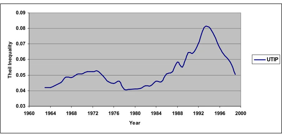
where Tw and TB indicate within-group and between-group inequality measures respectively. N and Y stand for total employment and total pay respectively, and subscript i denote group identity. TB is used as the inequality measure, where groups are defined as categories within the UNIDO industrial classification codes. Theil (1972) has shown that TB is a consistent lower-bound inequality measure, where the within-groups component is unobserved The UNIDO source permits calculation of inequality measures for nearly 3200 country/year observations, covering over 150 countries during the period 1963 to 1999. These measures were computed for the University of Texas Inequality Project.
are discarded from the calculations of EHII Gini coefficients. According to Galbraith and Kum (2004) EHII Gini has three clear advantages over the Deininger and Squire’s Gini index. First, with more than 3,000 estimates, the coverage basically matches that of the UTIP-UNIDO exercise, providing substantially annual estimates of household income inequality for most countries, including developing countries that are badly under-represented in D&S. Second, this data set borrows accuracy from the UTIP-UNIDO pay dispersion measures. Thus, changes over time and differences across countries in pay dispersion are reflected in income inequality, in proportion to their historical importance with due adjustment for the different employment weight of manufacturing in different economies. Third, all estimates are adjusted to household gross income hence data comparability across countries is greatly enhanced. Previously in this section we discussed the potential comparability problem that arises in D&S dataset as the unit of analysis varies between household and individuals, income used in calculating the gini is either in gross or net of value and lastly gini is calculated based either on income or expenditure. EHII dataset avoids this comparability issue by providing estimates which are adjusted to household gross income. However as mentioned in Section II, estimates based on gross household income may significantly overestimate the underlying inequality. Thus data comparability or homogenous method of reporting may come at a price.
As mentioned before the index is calculated from OLS estimates with conditioning variables, just two exogenous variables: pay inequality and manufacturing share, plus dummies for data type as described below.
In its log form the “EHII Gini” is simply:
EG = α + β * T + γ*X
III. Income Inequality and Explanatory Variables
A major part of this study is the presence of the conditioning variables. Major studies have shown that conditioning variables play a critical role in determining or unearthing the presence of Kuznets curve. Literature abounds with plethora of independent variables suspected to have influence on income inequality. Kuzents in his seminal paper did not specifically mention any independent variables as such and hence much of the one present in the literature are derived from an intuitive understanding of the way inequality works. However Kuznets did indicate few areas which will affect inequality and one may derive few variables in this regards. For instance he mentions that ‘An invariable accompaniment of growth in developed countries is the shift away from agriculture, a process usually referred to as industrialization and urbanization’ and in another place he states that ‘particularly so during the periods when industrialization and urbanization were proceeding apace and the urban population was being swelled’, therefore urban population or share of manufacturing sector in labor force may be a plausible independent variable and it has been used in Galbraith and Kum (2004).
We see similar conclusion being reached by Alderson and Nielsen (2002). As they suggest that inequality is attributable to differences in average income between sectors, which are called sector dualism and that sector dualism, is a function of the difference in average income between sectors and the relative size of the sectors. They use percentage of labor force in agriculture as a conditioning variable to capture this affect. In this paper we will also use the same variable. Data on the total agricultural labor force are estimated by FAO based on the close relationship existing between the ratio of economically active population in agriculture to the total economically active population and the ratio of agricultural population to total population. Annual figures are obtained through interpolating and extrapolating from the ILO decennial series6.
Since EHII dataset is developed with ratio of manufacturing employment to population as a conditioning variable, it is very likely that multicollinearity will exist if we use percentage of labor force in agriculture as the other conditioning variable. Therefore incase of EHII dataset we will use share of urban population instead of labor force in agriculture in order to capture the sector dualism, or industrialization as such. Estimates of the proportion of the population living in urban areas are obtained from national sources, such as censuses or population registers. Variations between countries make it nearly impossible to adopt uniform criteria for distinguishing urban from rural areas. As such, national statistical offices are often in the best position to establish appropriate criteria to characterize urban areas in their respective countries. 7
The relation between education and inequality still remains much unexplored. One of the primary reasons for this is the lack of global dataset. However, recently Barro and Lee (1993, 1995, 2001) have developed a global dataset for International measures of schooling years and schooling quality. In Alderson and Nielsen (2002), Gregorio and Lee (1999) they use secondary school enrollment ratio as a conditioning variable while analyzing the interrelationship between education and inequality. Also Barro and Lee (2001) themselves
6For more information, please see the FAO's Annual Series of Demographic Estimates explanatory notes.
suggest that the over-15 age group corresponds better to the labor force for many developing countries. The data set comprises at least one observation for 142 economies, of which 109 have complete information at five-year intervals from 1960 to 2000. Since the dataset are on a five year interval, linear interpolation was used to fill in the gap in the years in-between. Although this might result in serial correlation, since analysis will also be done on five year average dataset as well, this criticism may not be that severe. In this paper Percentage of "secondary school complete" in the total population was used as proxy for educational attainment, inline with current literature. However in this paper we will not look in to the relationship between educational inequality and income inequality although recent panel educational inequality dataset developed by Castelló and Doménech (2001) makes it possible. The author believes that further research can be carried out in this arena.
Demography has also been shown to have implications when it comes to inequality. Higgins and Williamson (2002) used cohort size as a conditioning variable and found that it has a significant impact on inequality. The cohort-size hypothesis is simple enough: fat cohorts tend to get low rewards. When those fat cohorts lie in the middle of the age-earnings curve, where life-cycle income is highest, this labor market glut lowers their income, thus tending to flatten the age earnings curve. Earnings inequality is moderated. When instead the fat cohorts are young or old adults, this kind of labor market glut lowers incomes at the two tails of the age-earnings curve, thus tending to heighten the slope of the upside and the downside of the age-earnings curve. Earnings inequality is augmented. In their paper they used the variable MATURE to capture this effect and the variable was defined to be the proportion of the adult population who are 40-59. In the current paper the variable is further segregated to include the proportion of adult female and male population who are 40-59, thus bringing an additional gender dimension to the study. The data is taken from United Nations Statistics Division, UNSD, Demographic Statistics.
contestable area. At the same time, increasing opportunities to trade are likely to affect income distribution and whether or not increasing openness to trade is accompanied by a reduction or an increase inequality is highly controversial. The usual hypothesis is developing countries have an abundant supply of unskilled labor relative to skilled labor and developed countries have an abundant supply of skilled labor relative to unskilled labor. Hence increased openness in developing countries is assumed to boost the relative demand for skilled labor which in turn will increase overall inequality, all else being equal. However results remain much less clear cut. In the following page there is a snapshot of major studies done so far on inequality and openness relationship. What becomes clear is that results are far from conclusive. In this paper we use total trade as a percentage of GDP as defined by openk variable in Penn World Table 6.2.
Table 2: Studies on openness and inequality8
The final variable is the standard real GDP per capita/worker which is the most widely used indicator for capturing the Kuznets effect Deininger and Squire (1998), Barro (2000), RAM (1991, 1997), Frazer (2006), Higgins and Williamson (2002) etc . Although whether to use its level or log form remains to be decided. In this paper we will use real GDP per capita/worker (in constant 1996 US$) Penn World Tables dataset, version 6.2. In some paper, particularly Higgins and Williamson (2002) use per worker instead of the usual per capita and hence both will be used in this study.
In the literature we also find other interesting variables which have been shown to influence income inequality. For instance in Bahmani-Oskooee, Goswami, Mebratu (2006) it was shown that income inequality is higher in countries that have black market for foreign exchange. While in Chong (2004) it was found that democracy has non-monotonic link with income inequality. However in this paper we will restricts ourselves to conditioning variables discussed in Higgins and Williamson (2002), since the paper was found to be significantly broad in scope in terms of its coverage of conditioning variables. In some cases slight variation will be used, for instance we will employ gender segregated matured cohort size instead of the mature adult cohort size, which was not gender segregated , as was used in Higgins and Williamson (2002). In case of EHII we will use share of urban population, which was not mentioned in Higgins and Williamson (2002) but this is done to avoid multicollinearity issue. But nonetheless the current paper draws heavily, in terms of choice of explanatory variables, from Higgins and Williamson (2002) specifically their extended regression model.
Table 3: Relevant Variables and Labels
Variables Label
gdp_pc Real GDP per capita
gdp_wc Real GDP per worker
recgdp_pc Reciprocal of Real GDP per capita recgdp_wc Reciprocal of Real GDP per worker
lngdpc Ln of Real GDP per capita
lngdpc2 Square of Ln of Real GDP per capita
lngdpw Ln of Real GDP per worker
lngdpw2 Square of Ln of Real GDP per worker
openk Trade Openness
labor_agri Percentage of labor force in agriculture
U_Pop Share of urban population
Edu_Sec_15 Percentage of secondary school complete lnedu Ln of Percentage of secondary school complete male4059 Proportion of the male population who are 40-59 female4059 Proportion of the female population who are 40-59
wiid2 World Income Inequality dataset ehii Estimated Household income inequality dataset utip UTIP UNIDO Manufacturing Pay inequality
IV.
Econometric issues Panel Unit root tests
At one time, conventional wisdom was that in order to apply standard inference procedures in such studies, the variables in the system needed to be stationary since the vast majority of econometric theory is built upon the assumption of stationarity. Consequently, for many years econometricians proceeded as if stationarity could be achieved by simply removing deterministic components (e.g., drifts and trends) from the data. However, stationary series should at least have constant unconditional mean and variance over time, a condition which hardly appears to be satisfied in economics, even after removing those deterministic terms. Yule (1926) pointed out that spurious correlation may persist in large sample despite the absence of any connection between the underlying series.
Therefore before we undertake any econometric analysis we must first need to ascertain the order of integration for all the variables, dependent and independent. If all the variables are stationary then we can perform econometric analysis without being concerned about the possibility of spurious regressions and inappropriate standards errors. However, some variables may possess unit root and therefore be mean or variance non stationary. In such cases either we need to difference the variable (mean non stationary) and/or log transformed the series (variance non stationary). In order to address the issue of stationarity of the variables, we undertake panel unit root tests
All the tests are primarily based on the following ADF specification:
Here, represents the country specific fixed effects and unit specific linear time trends respectively. For LLC and BR tests, it is assumed that Hence, the null hypothesis of a unit root translates to . The IPS, PP and ADF tests allow the autoregressive coefficient to vary across countries which entails the alternative hypothesis as . Therefore, the reported t-statistic is the sample-weighted average of the t-statistics for the individual countries.
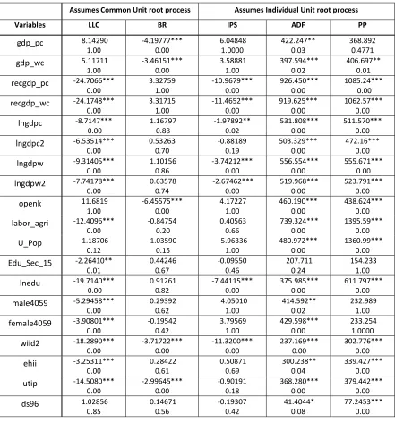
Table 4: Panel Unit Root test
Assumes Common Unit root process Assumes Individual Unit root process
Variables LLC BR IPS ADF PP
gdp_pc 8.14290
1.00 -4.19777*** 0.00 6.04848 1.0000 422.247** 0.03 368.892 0.4771
gdp_wc 5.11711
1.00 -3.46151*** 0.00 3.58881 1.00 397.594*** 0.02 406.697** 0.01
recgdp_pc -24.7066***
0.00 3.32759 1.00 -10.9679*** 0.00 926.450*** 0.00 1085.24*** 0.00
recgdp_wc -24.1748***
0.00 3.31715 1.00 -11.4652*** 0.00 919.625*** 0.00 1062.57*** 0.00
lngdpc -8.7147***
0.00 1.16797 0.88 -1.97892** 0.02 531.808*** 0.00 511.570*** 0.00
lngdpc2 -6.53514***
0.00 0.53263 0.70 -0.88189 0.19 503.329*** 0.00 472.16*** 0.00
lngdpw -9.31405***
0.00 1.10156 0.86 -3.74212*** 0.00 556.554*** 0.00 555.671*** 0.00
lngdpw2 -7.74178***
0.00 0.63578 0.74 -2.67462*** 0.00 519.968*** 0.00 523.791*** 0.00
openk 11.6819
1.00 -6.45575*** 0.00 4.17227 1.00 460.190*** 0.00 438.624*** 0.00
labor_agri -12.4096***
0.00 -0.84754 0.20 0.40563 0.66 739.324*** 0.00 1395.59*** 0.00
U_Pop -1.18706
0.12 -1.03590 0.15 5.96336 1.00 480.972*** 0.00 1360.99*** 0.00
Edu_Sec_15 -2.26410**
0.01 0.44246 0.67 -0.09550 0.46 207.711 0.24 154.233 1.00
lnedu -19.7140***
0.00 0.91261 0.82 -7.44115*** 0.00 375.985*** 0.00 611.797*** 0.00
male4059 -5.29458***
0.00 0.29392 0.62 4.05010 1.00 414.592** 0.02 232.989 1.00
female4059 -3.90801***
0.00 -0.19542 0.42 3.79569 1.00 429.598*** 0.00 233.254 1.0000
wiid2 -18.2890***
0.00 -3.71722*** 0.00 -11.3200*** 0.00 237.169*** 0.00 302.776*** 0.00
ehii -3.25311***
0.00 0.28422 0.61 0.50871 0.69 300.238** 0.04 339.427*** 0.00
utip -14.5080***
0.00 -2.99645*** 0.00 -0.90191 0.18 368.280*** 0.00 379.442*** 0.00
ds96 1.02856
0.85 0.14671 0.56 -0.19307 0.42 41.4044* 0.08 77.2453*** 0.00
capita and 1/(real GDP per capita)) is not justified and neither is the form real GDP per capita and square of real GDP per capita, as used by others. Unless of course one can show that a cointegrating relationship exists between these variables and the inequality variable, in which case spurious relationship can be avoided. Since the log transformed form of both real GDP per capita and real GDP per worker, along with their quadratic form, perform consistently better than their level form, we will use them in this paper, in line with Barro (2000).
Other than the real GDP per capita, the rest of variables give a mixed result but in most cases 3 of the tests at least show the other variables to be stationary. Only in case of Percentage of secondary school complete, Edu_Sec_15, do we see gross violation of unit root test. However we see that the log transformed form performs much superiorly. Hence we can see that in its level form, like real GDP per capita and real GDP per worker, the variable is variance non-stationary. In this paper we are going to use the log transformed form.
Since the objective of the study is testing the robustness of the Kuznets hypothesis, much greater emphasis will be given on the real GDP per capita and real GDP per worker. Therefore in reference to conditioning variables, even at the chance of receiving criticism, the author believes that the variables are satisfactorily stationary and hence no further transformation will be carried out. Thus the functional form we end at is
INEQit = αi + β1 (lnYit)+ β2(lnYit)2 + βi Xit + εit (1).
Where INEQit is the inequality measure (WIID2, UTIP, EHII, DS) , αi is the country
specific fixed effect9 , lnYit is Real GDP per capita or worker and Xit is the constellation of conditioning variables, namely Trade Openness, Percentage of labor force in agriculture or Share of urban population, Ln of Percentage of secondary school complete, Proportion of the male population who are 40-59 and Proportion of the female population who are 40-59.
9Most research done after early 90s use Fixed effect modeling, Deininger and Squire (1998), Ram (1991 1997), Barro
V.
Alternative Estimation of Inequality Relationship
Previous studies on inequality and development studies used crosssection or pooled datasets. Naturally, what we want to understand is how inequality changes over time, or with level of development, within a country, and yet, because of previous data limitations, the empirical tests were forced to draw conclusions largely from cross-sectional (or pooled) datasets. But with the advent of D&S, 1996 this problem has been significantly mitigated, if not completely so. In this paper we will use D&S, 1996 inequality dataset, along with three other datasets10 , which also have panel structure. In line with existing literature11 we will initially undertake pooled regression on the three types of dataset, namely Annualized global dataset of 188 countries, 4 year average of global dataset and OECD datasets. This is the simplest form of analysis and after that we will undertake specification tests to see whether pooled or random effect or fixed effect modeling is appropriate. We will also try to refine our modeling to ensure that there is no misspecification error or serial correlation. Therefore pooled regression is done to enhance the comparability of present research with earlier research.
Pooled Regression
In this section we will try to develop the econometric model in order to investigate the shape and existence of Kuznets curve using the explanatory variables mentioned in the previous section. We will run regression on the annualized global dataset, 4 years average dataset and finally on the OECD section of the annualized dataset, as much research has been done on investigating inequality relationship for OECD countries. The following table gives the result of pooled regression for the three types of dataset and the 4 different inequality measures.
10 World income inequality database (WIID2), UTIP UNIDO Manufacturing Pay inequality dataset (UTIP), and
Estimated Household Income Inequality Data Set (EHII)
Table 5: Pooled regression on annualized dataset, all countries
Dependent Variable
Regressor DS96 WIID2 EHII UTIP UTIP-W
c -86.271*** 0.00 -38.562* 0.08 83.077*** 0.00 0.612* 0.00 0.756* 0.00
lngdpc 26.610*** 0.00 20.645*** 0.00 -5.676*** 0.00 -0.111** 0.00
lngdpc2 -1.033** 0.01 -0.914*** 0.00 0.328*** 0.00 0.007*** 0.00
openk 0.0158** 0.05 0.012*** 0.01 0.007*** 0.00 8.14E-05*** 0.00 7.36E-05*** 0.00
labor_agri 0.173*** 0.00 0.001 0.97 -8.70E-05*** 0.39
-0.00036***
0.00
u_pop -0.053*** 0.00
lnedu -1.346** 0.00 -2.867*** 0.00 -0.324** 0.02 -0.001 0.42 -0.001 0.49
male4059 -3.007*** 0.00 -4.577*** 0.00 -0.634*** 0.01 0.012*** 0.00 0.011*** 0.00
female4059 0.693 0.11 1.773*** 0.00 -0.105 0.42 -0.010*** 0.00 -0.01*** 0.00
lngdpw -0.123** 0.00
lngdpw2 0.006*** 0.00
Cross section 74 87 93 93 93
N 469 1094 2307 2284 2281
Adj R-squared 0.57 0.49 0.57 0.22 0.22
DW stat 0.52 0.56 0.14 0.33 0.34
F-statistic 89.01 152.26 438.50 92.18 95.47
Prob(F-stat) 0.00 0.00 0.00 0.00 0.00
multicollinearity issue and we see that it has negative coefficient. This is also counter intuitive as increased urbanization should increase inequality and not decrease it. However we see in some cases it is not significant. Once fixed effect model is run, one needs to monitor the effect it has on this variable. In case of Galbraith Kum we see that fixed effect may wash away the significance of urbanization or such variables. Hence further analysis should be deferred till that time. Education variable is negative in all cases, although in case of UTIP it is not significant. It is in line with literature as education is considered to be one of the key leveling factors which reduce inequality.
Gender segregated cohort size show a very interesting result. In case of D&S and WIID2, male cohort has a negative coefficient while positive for female. In accordance with Williamson Higgins (2002) finding large mature working-age cohorts are associated with lower aggregate inequality, which seems to hold for male cohort size and goes in opposite direction when it comes to females’ cohort size. It is very interesting as one over the last 20-30 years female participation in the labor force has increased significantly. Hence in coming decade, worldwide, there will be a significant proportion of matured female labor force. In EHII both coefficient are negative but in case of female it is insignificant. But in case of UTIP the signs are reversed with Male cohort size being positive and negative in case of female. It could be attributed to the fact that the dynamics of inequality within manufacturing sector may differ from that of overall country inequality dynamics but it is an area which surely needs further investigation.
Table 6: Pooled regression on Average dataset
Due to lack of data points after averaging for 4 years, it was not possible to carryout regression for D&S dataset. What becomes clear from above tables is that the Kuznets curve still does not appear for UTIP or EHII dataset while it is clearly seen in case of WIID2 and D&S (OECD). This is an important finding because in Galbraith and Kum (2004) it is mentioned that ‘For the OECD countries (Western Europe and North America) where the direct measurement of household income inequality is likely to be most advanced and most consistent, there is not much systematic divergence between the two data sets’- EHII and D&S. this might be true in case of descriptive statistics but in case regression analysis the results are still divergent. Similarly results are divergent with WIID2 dataset which is a much improved version of D&S 1996. Further analysis on this disparity will be carried out in the later part. The coefficient values of the quadratic and the linear term of per capita income significantly increases for all datasets.
In terms of independent variables we see divergence emerge among the findings of dataset for OECD countries. In case of openness, there is strong negative relationship with inequality
Dependent Variable
Regressor WIID2 EHII UTIP UTIP-W
c
-23.519 85.614*** 0.611*** 0.781***
0.44 0 0 0
lngdpc
17.789*** -6.222** -0.108***
0.01 0.05 0
lngdpc2
-0.790** 0.363* 0.006***
0.05 0.06 0
openk
0.019** 0.008** 0.0001*** 0.0001***
0.02 0.04 0.01 0.01
labor_agri
0.006
0.0002 -0.0005**
0.88 0.4 0.02
u_pop
-0.052***
0
lnedu
-3.003*** -0.266 -0.001 -0.0006
0 0.28 0.71 0.82
male4059
-2.752*** -0.618 0.013*** 0.015***
0 0.16 0 0
female4059
0.745 -0.133 -0.010*** 0.0113***
-0.14 0.59 0 0
lngdpw -0.122*** 0 lngdpw2 0.006*** 0
Cross section 88 93 93 93
N 492 646 640 640
Adj R-squared 0.48 0.57 0.21 0.22
DW stat 0.59 0.3 0.5 0.5
F-statistic 65.53 124.62 25.47 27.21
in case of WIID2 and D&S dataset, while it is just the opposite in case of EHII and UTIP. In case of labor participation in agriculture, the coefficient value remains positive for all dataset. It might be hypothesized that because of the modernization and mechanization of agriculture in OECD countries the increase in labor force participation in the sector may actually increase inequality. Also the sector may not be as unionized as the manufacturing sector and hence leveling effect may be missing.
Table 7: Pooled regression on OECD dataset
Dependent Variable
Regressor DS96 WIID2 EHII UTIP UTIP-W
c
-84.798 -265.475*** 247.760*** 0.2511** 0.4171**
0.14 0 0 0.03 0.02
lngdpc
13.7518 57.819*** -44.899*** -0.0659***
0.26 0 0 0.01
lngdpc2
-0.1129 -2.633*** 2.455*** 0.0044***
0.87 0 0 0
openk
-0.0552*** -0.058*** 0.011** 0.0001*** 0.0001***
0 0 0.04 0 0
labor_agri
0.4556*** 0.320***
0.0008*** 0.0007***
0 0 0 0
u_pop
-0.086***
0
lnedu
0.6352 0.165*** -0.835*** -0.0046*** -0.0039***
0.17 0.74 0 0 0
male4059
-1.5573*** -2.980*** -1.528*** -0.0049*** -0.0055***
0.01 0 0 0 0
female4059
0.6517* 1.339*** 0.847*** 0.0027*** 0.0031***
0.07 0 0 0 0
lngdpw -0.0954*** 0.01 lngdpw2 0.0055*** 0
Cross section 21 23 22 23 23
N 238 495 744 748 748
Adj R-squared 0.45 0.26 0.24 0.21 0.2
DW stat 0.17 0.53 0.05 0.17 0.17
F-statistic 28.83 25.23 35.2 28.8 27.74
Prob(F-stat) 0 0 0 0 0
inequality in developed countries is higher in areas outside urban locale. Now this may be due to the fact that most of the factories/manufacturing units are outside urban areas due to high real estate cost, hence urbanization may not necessarily imply industrialization. It may also mean that in developed countries agriculture has higher inequality. This may explain the positive relationship between agricultural labor participation, urbanization and inequality.
In case of cohort size we see a consensus between all datasets and the gender dimension becomes even more pronounced. As the size of matures female working population increases inequality decreases and vise versa for male. This may actually stem from the fact that incase of female the wage/income differential is not as high as in the case for male. This egalitarian income differentiation among female may actually be a result of gender discrimination rather than homogenous skill sets among female which thus fetches similar wages/income. Since the current matured population entered the labor force when gender discrimination may still have been prevalent, it is very likely that employment opportunity for woman back then were less in comparison to male. Hence wage/income for the current female population is similar and hence the coefficient value is negative. If this is indeed the case then in future this difference between male and female mature working population will diminish and may even disappear. In case of OECD countries the sign reverses and it seems now increasing size of female population increases inequality while decreases it in the case of male. Could it be due to the fact that OECD countries have tried to mainstream gender and in the process have selectively focused on high skilled female labors in order to set up example for future generation or could it be that the limited opportunities available to female covered opposite areas of the income spectrum. Hence a female could either enter as secretary or business executive resulting in current high inequality among current female matured workforce. This area requires further investigation and may provide some interesting findings in future research.
terms of labor participation in agriculture and urbanization is still prevalent. The only significant difference arises in the DW statistics which improves slightly, indicating that serial correlation may not necessarily stem only from the linear interpolation used in case of some independent variables. Hence different econometric method must be employed to remove the problem of serial correlation, dynamic panel or inclusion of AR1 may be used.
In case of UTIP in one case we use per capita income and its square, while in the other case, UTIP-W, we used per worker and its square. From the above tables we see that the sign and the coefficient value for the per capita and per worker do not change significantly to warrant running separate set of regressions for per worker. The sign of the coefficient and values for independent variables also do not change much. Therefore in the following sections we will limit our study to per capita income, excluding per worker, and will only focus on annualized and OECD datasets, excluding average dataset.
Fixed effect Regression
After running pooled regression, two formal specification tests are performed. One is Breusch and Pagan’s LM test (1980), to see the relevance of random-effects specification; If the test statistic, based on chi square distribution, rejects the null hypothesis (which it does in this case), then a random effects model is regarded as preferable. The other test is a Hausman test for specification (1978). The null hypothesis in this test is that country-specific effects are not correlated with any regressor in the model equation, implying that the estimates are efficient. If this null is rejected, the random effects model estimates are inconsistent and fixed effects model specification would be preferred. Test results show that a random-effects model provides inconsistent estimates in equation (1).
section we will initially test unconditional Kuznets hypothesis, before proceeding in to testing the conditional Kuznets hypothesis with all the explanatory variables.
Table 8: Fixed effect regression for Unconditional Kuznets curve on Annualized all countries
In the above table we see that the difference between WIID2 and EHII continues, with Kuznets hypothesis being confirmed in case of first measure of inequality while being rejected in case of the second. In case of D&S and UTIP although both confirm Kuznets hypothesis however the coefficient values are not significant. The following table shows the result for OECD countries.
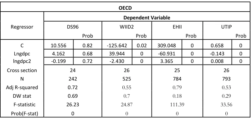
Table 9: Fixed effect regression for Unconditional Kuznets curve on OECD countries
OECD
Dependent Variable
Regressor DS96 WIID2 EHII UTIP
Prob Prob Prob Prob
C 10.556 0.82 -125.642 0.02 309.048 0 0.658 0
Lngdpc 4.162 0.68 39.944 0 -60.931 0 -0.143 0
lngdpc2 -0.199 0.72 -2.430 0 3.365 0 0.008 0
Cross section 24 26 25 26
N 242 525 784 793
Adj R-squared 0.72 0.55 0.79 0.53
DW stat 0.69 0.7 0.18 0.29
F-statistic 26.23 24.87 111.39 33.56
Prob(F-stat) 0 0 0 0
Global Dataset
Dependent Variable
Regressor DS96 WIID2 EHII UTIP
Prob Prob Prob Prob
c 18.389 0.42 -12.996 0.50 87.986 0 -0.126 0.28
lngdpc 4.596 0.39 13.799 0.00 -10.622 0 0.043 0.11
lngdpc2 -0.277 0.38 -0.881 0.00 0.603 0 -0.002 0.11
Cross section 107 139 145 146
N 575 1442 2892 2901
Adj R-squared 0.9 0.78 0.86 0.62
DW stat 0.93 0.9 0.42 0.91
F-statistic 51.4 37.99 121.67 32.59
[image:36.612.115.516.525.715.2]In case of OECD dataset we see that the difference in finding continues to persist between WIID2 inequality measure and EHII measure. However in case of OECD countries, coefficient values become significant for both UTIP and D&S but the difference remains, with D&S confirming Kuznets curve while UTIP rejects it. The finding are in consensus with Munir and Muaz (2004) where an un-inverted U shaped curve was found, while for testing unconditional Kuznets curve, in case of both UTIP and EHII dataset. Munir and Muaz (2004) carried out the study on a balanced panel of 24 countries. In the following page we run fixed effect model on conditional Kuznets curve to further analyze the issue.
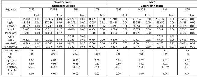
Table 10: Fixed effect regression on Annualized all countries and OECD dataset
Global Dataset OECD
Dependent Variable Dependent Variable
Regressor DS96 WIID2 EHII UTIP DS96 WIID2 EHII UTIP
Prob Prob Prob Prob Prob Prob Prob Prob
c -75.098 0.01 -79.475 0.00 129.777 0.00 0.399 0.00 -292.041 0.00 -397.167 0.00 293.272 0.00 0.705 0.00
lngdpc 18.453 0.01 27.286 0.00 -20.276 0.00 -0.050 0.11 55.630 0.00 85.738 0.00 -55.650 0.00 -0.139 0.00
lngdpc2 -0.822 0.03 -1.738 0.00 1.027 0.00 0.001 0.56 -2.493 0.00 -4.554 0.00 2.904 0.00 0.007 0.00
openk 0.042 0.00 -0.014 0.17 -0.010 0.00 0.000 0.00 0.079 0.05 -0.075 0.00 0.093 0.00 0.000 0.00
labor_agri 0.291 0.00 0.054 0.17 -0.001 0.00 0.754 0.00 0.499 0.00 0.000 0.07
u_pop 0.088 0.00 0.027 0.43
lnedu -0.185 0.66 -0.312 0.48 0.732 0.00 0.010 0.00 0.170 0.77 1.822 0.01 -0.604 0.00 -0.005 0.00
male4059 -0.249 0.67 -1.986 0.00 -0.192 0.37 -0.001 0.64 0.105 0.87 -1.681 0.01 -0.275 0.15 -0.001 0.34
female4059 0.263 0.44 1.567 0.00 0.245 0.04 0.002 0.27 0.167 0.65 1.470 0.00 0.232 0.03 0.001 0.32
Cross section 74 87 93 93 21 23 22 23
N 469 1094 2307 2284 238 495 744 748
Adj
R-squared 0.92 0.80 0.86 0.61 0.78 0.57 0.83 0.59
DW stat 0.90 0.94 0.36 0.62 0.80 0.82 0.23 0.34
F-statistic 68.03 49.47 136.37 37.06 31.23 23.48 134.59 38.08
In case of openness the results are rather mixed and are no longer as straightforward as before. To begin with we see that in case of D&S for Global Dataset the coefficient is positive, insignificant for WIID2 and negative for EHII . But in case of OECD we see that there is a disagreement between WIID2 and D&S dataset, which may be of interest. For labor participation in agriculture the result remains consistent with the previous counter intuitive result. Education is significant mostly for EHII and UTIP dataset. In the annualized dataset it has a positive coefficient while in case of OECD it is negative. One may attribute this to the fact that annualized Global Dataset, especially EHII and UTIP, has a greater representation of developing LDC countries and in these countries return to education may be very high. Hence at the initial stages of development higher secondary level education attainment may increase inequality as the skill set demanded in the developing labor market may not be that high. In OECD countries education may play the role of leveling effect and return to education might be lower, which reduces inequality. In case of cohort size the gender dimension with negative sign for male cohort still persists although in some cases, especially in OECD dataset, it looses significance. But this time we see across both OECD and Global Dataset that mature male population tend to reduce inequality while female tend to increase it.
Fixed effect Regression with AR1 error
It is also seen that there is significant improvement in Adjusted R-squared value and DW statistics for both regressions under both dataset. However this is very likely the result of country specific constant which is boosting the explanatory power of the regression without enhancing the interpretive power of the regression in any significant way. There is still serial correlation as the DW statistics is still very low. In equation (1) the error term (εit) is naively
supposed to be white noise, satisfying the standard I.I.D.~(0,σ2) assumption. However, his is
(1999), which can deal with unbalanced panel structure of our data. Then the equation (1) is modified as
INEQit = αi + β1 (lnYit)+ β2(lnYit)2 + βi Xit + εit (2)
Where εit = ρεit-1 +ηit
where ρ is a correlation coefficient among (εit , εit-1) and ηit is again conventional white noise satisfying the I.I.D.~(0,σ2) assumption.
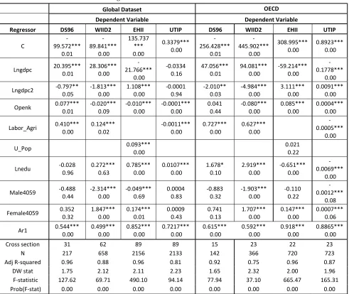
Table 11: Fixed effect regression on annualized all countries and OECD dataset with AR1
Global Dataset OECD
Dependent Variable Dependent Variable
Regressor DS96 WIID2 EHII UTIP DS96 WIID2 EHII UTIP
C 99.572***
-0.01 -89.841*** 0.00 135.737 *** 0.00 0.3379*** 0.00 -256.428*** 0.01 -445.902*** 0.00 308.995***
0.00 0.8923*** 0.00
Lngdpc 20.395*** 0.01 28.306*** 0.00 21.766*** 0.00
-0.0334
0.16 47.056*** 0.01 94.081*** 0.00 -59.214*** 0.00 -0.1778***
0.00 Lngdpc2 -0.797** 0.05 -1.813*** 0.00 1.108*** 0.00 -0.0001 0.94 -2.010** 0.03 -4.984*** 0.00 3.111*** 0.00 0.0091*** 0.00
Openk 0.077*** 0.01 -0.020*** 0.09 -0.010*** 0.00 -0.0001*** 0.00 0.041 0.44 -0.080*** 0.00 0.085*** 0.00 0.0004*** 0.00
Labor_Agri 0.410*** 0.00 0.124*** 0.02 -0.0011*** 0.00 0.727*** 0.00 0.627*** 0.00 0.0005*** 0.00
U_Pop 0.093*** 0.00 0.021 0.22
Lnedu -0.028 0.96 0.272*** 0.63 0.785*** 0.00 0.0107*** 0.00 1.678* 0.10 2.919*** 0.00 -0.651*** 0.00 0.0069*** 0.00
Male4059 -0.488 0.44 -2.314*** 0.00 -0.049*** 0.69 0.0004 0.83 -0.883 0.32 -1.903*** 0.00 -0.110 0.22 0.0012*** 0.08 Female4059 0.352 0.32 1.847*** 0.00 0.174*** 0.01 0.0009 0.43 0.741 0.13 1.707*** 0.00 0.147*** 0.00 0.0007*** 0.06
Ar1 0.544*** 0.00 0.499*** 0.00 0.852*** 0.00 0.7217*** 0.00 0.615*** 0.00 0.592*** 0.00 0.918*** 0.00 0.8865*** 0.00
Cross section 31 62 89 89 15 23 22 23
N 217 658 2156 2133 142 366 720 723
Adj R-squared 0.96 0.88 0.96 0.81 0.92 0.75 0.96 0.87
DW stat 1.75 2.12 2.11 2.23 1.65 2.32 2.00 1.96
F-statistic 127.62 69.71 490.10 94.14 77.94 37.10 665.47 165.31
Prob(F-stat) 0.00 0.00 0.00 0.00 0.00 0.00 0.00 0.00
In case of openness, although the coefficient value changes somewhat but the sign remains more or less consistent with previous fixed effect regression result. For the standard annualized dataset the signs are positive for D&S dataset but negative for the rest. While in case of OECD, the coefficient value and sign becomes more robust for WIID2 but changes significantly for UTIP and EHII, both in terms of sign and value.
For participation of labor force in agriculture, for both OECD and annualized dataset the coefficient is positive and highly significant. However UTIP shows a negative sign in case of Global Dataset and OECD datasets. So the disparity in findings for the dataset continues. For urbanization, coefficient is positive but insignificant in case of OECD.
The variable of secondary education attainment shows positive coefficient for EHII and UTIP in case of Global Dataset but significant and negative for OECD countries, which may be due to the fact, as mentioned before, that Global Dataset has greater proportion of LDCs and developing countries where the return to education is higher than OECD, hence education tend to increase inequality. For WIID2 and D&S dataset, the variable is insignificant in Global Dataset but becomes significant and positive in case of OECD countries and this finding obviously puts to question the aforementioned reason for negative sign in case of EHII and UTIP dataset in OECD countries. Which result is valid can only be answered if one can suggest or choose a dataset over the other thereby invalidating the findings of the other dataset
For Cohort size we see that Female factor remains significant in case of WIID2 for both standard and OECD dataset and it is positive, while male cohort size is negative and is also significant. Female cohort size is significant in case of EHII for both dataset and is also positive. But one thing that becomes clear is that after the inclusion of AR1, which is significant at 1% level in all cases, apart from WIID2 in all other cases it is negative but insignificant12. The DW statistics shows significant improvement after the addition of AR1 term, as was expected.
However serial correlation may arise in residuals (εit) from another source, that is, from some
influence of omitted lagged dependent variables, then not only could standard errors of the estimates but also coefficient estimates be biased. This is a plausible suspicion, because the previous year’s inequality could have some persistency in determining the current year’s inequality. If this were the case, the previous remedy focused on only the error term would not generate a reliable result. To address this problem, a lagged dependent variable (LDV) specification is adopted. Then equation (1) can be modified as
INEQit = αi + γ1* INEQi(t-1) +β1 (lnYit)+ β2(lnYit)2 + βi Xit + εit (3)
estimates, the lagged dependent variable [INEQi(t-1)] should not be correlated with current error term: E(INEQi(t-1), εit) = 0 and the time dimension (t) should be expanded to infinity,
which is particularly not feasible in this study. To deal with this problem the popular method suggested by Arellano and Bond (1991) is adapted, which corrects the lagged dependent variable bias as well as permits a certain degree of endogeneity in the other regressors. This Generalized Method of Moment (GMM) estimator modifies our model by specifying a first-difference form, eliminating country-specific effects first, and uses the lagged value of each differenced term as instruments. Model (4) can be rewritten as
[INEQit- INEQi(t-1)] = γ1*[ INEQi(t-1) - INEQi(t-2)] + β1*[LnYit - LnYit-1]+ β2*[(ln Yit)2 -(ln Yit-1)2 ] + βi
*[ Xit - Xit-1] + [εit - εit-1] (4)
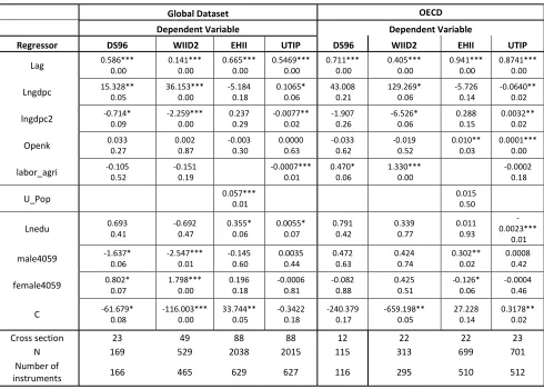
Table 12: Arellano-Bond on annualized all countries and OECD dataset
Global Dataset OECD
Dependent Variable Dependent Variable
Regressor DS96 WIID2 EHII UTIP DS96 WIID2 EHII UTIP
Lag 0.586*** 0.00 0.141*** 0.00 0.665*** 0.00 0.5469*** 0.00 0.711*** 0.00 0.405*** 0.00 0.941*** 0.00 0.8741*** 0.00
Lngdpc 15.328** 0.05 36.153*** 0.00 -5.184 0.18 0.1065* 0.06 43.008 0.21 129.269* 0.06 -5.726 0.14 -0.0640** 0.02
lngdpc2 -0.714* 0.09 -2.259*** 0.00 0.237 0.29 -0.0077** 0.02 -1.907 0.26 -6.526* 0.06 0.288 0.15 0.0032** 0.02
Openk 0.033 0.27 0.002 0.87 -0.003 0.30 0.0000 0.63 -0.033 0.62 -0.019 0.52 0.010** 0.03 0.0001*** 0.00
labor_agri -0.105 0.52 -0.151 0.19 -0.0007*** 0.01 0.470* 0.06 1.330*** 0.00 -0.0002 0.18
U_Pop 0.057*** 0.01 0.015 0.50
Lnedu 0.693 0.41 -0.692 0.47 0.355* 0.06 0.0055* 0.07 0.791 0.42 0.339 0.77 0.011 0.93 0.0023*** 0.01
male4059 -1.637* 0.06 -2.547*** 0.01 -0.145 0.60 0.0035 0.44 0.472 0.63 0.424 0.74 0.302** 0.02 0.0008 0.42
female4059 0.802* 0.07 1.798*** 0.00 0.196 0.18 -0.0006 0.81 -0.082 0.88 0.425 0.51 -0.126* 0.06 -0.0004 0.46
C -61.679* 0.08 -116.003*** 0.00 33.744** 0.05 -0.3422 0.18 -240.379 0.17 -659.198** 0.05 27.228 0.14 0.3178** 0.02
Cross section 23 49 88 88 12 22 22 23
N 169 529 2038 2015 115 313 699 701
Number of
instruments 166 465 629 627 116 295 510 512
VI.
Analysis
After going through the above procedure some of the key findings are mentioned below –
1. Kuznets curve is evident when dependent variable is WIID2 and D&S and an un-inverted curve is found when inequality is EHII. This finding is independent of controlling variable and the econometric model used (pool, fixed, autoregressive fixed effect, dynamic panel)
2. Relationship between openness and inequality is not clear cut and varies based not only on choice of dependent variable but also on the econometric model used
3. Labor participation in agriculture seems to have a positive relationship with inequality especially in case of OECD countries. The finding is in stark opposition to that found in current literature and what Kuznets hypothesized where agriculture was assumed to have lower level of income inequality.
4. Other than pooled regression, in other cases (fixed, autoregressive fixed effect, dynamic panel) urbanization has a significant, especially for Global Dataset, positive relationship with inequality. This is pretty much in line with findings in literature and Kuznets hypothesis, which states that greater urbanization should lead to higher inequality.