Munich Personal RePEc Archive
GMM estimation of spatial panels
Moscone, Francesco and Tosetti, Elisa
Brunel University
17 April 2009
Online at
https://mpra.ub.uni-muenchen.de/16327/
GMM estimation of spatial panels
F. Moscone
yBrunel Business School
E. Tosetti
zUniversity of Cambridge
Abstract
We consider Generalized Method of Moments (GMM) estimation of a regression model with spatially correlated errors. We propose some new moment conditions, and derive the asymptotic distribution of the GMM based on them. The analysis is supported by a small Monte Carlo exercise.
Keywords: Generalized Method of Moments, spatial econometrics.
JEL Code: C2, C5.
1
Introduction
GMM estimation of spatial regression models has been originally advanced by Kelejian and Prucha (1999). They suggested three moment conditions that exploit the properties of disturbances implied by a standard set of assumptions. Substantial work has followed their original study. Druska and Horrace (2004) have considered GMM estimation of a panel regression with time dummies and time-varying spatial weights. Lee and Liu (2006a) suggested a set of linear and quadratic moment conditions in the errors with inner matrices satisfying certain regularity properties; Lee and Liu (2006b) have extended this framework to estimate regression models with higher-order spatial lags. Fingleton (2008a) and Fingleton (2008b) proposed a GMM estimator for spatial regression models with an endogenous spatial lag and moving average errors. Kelejian and Prucha (2008) have generalized their original work to allow heteroskedasticity and spatial lags in the dependent variable. This has been extended by Kapoor et al. (2007) to estimate a spatial panel regression with individual-speci…c error components.
We focus on GMM estimation of a regression model where the error follows a spatial autoregressive (SAR) process. We show that there are more moments than those currently exploited in the literature, and derive the asymptotic distribution of the GMM based on such moments. We perform a small Monte Carlo exercise to compare the properties of GMM estimators based on di¤erent sets of moments.
2
The framework
Consider the model expressed in stacked form
yt = Xt +ut; t= 1; :::; T; (1)
ut = Sut+"t; (2)
where yt = (y1t; :::; yN t)0,Xt = (x1t; :::;xN t)0,ut = (u1t; :::; uN t)0, "t = ("1t; :::; "N t)0 and S is N N spatial
weights matrix. We assume:
The authors acknowledge …nancial support from ESRC (ref. no. RES-061-25-0317). We have bene…ted from comments by the partecipants of the III World Spatial Econometrics Association.
Assumption 1: "it IIDN(0; 2), with 2 K <1, fori= 1; :::; N; t= 1; :::; T.
Assumption 2: Xtand"t0 are independently distributed for allt; t0. AsN and/orT ! 1N T1 PTt=1X0tXt!
M, where Mis …nite and non-singular.
Assumption 3: Shas zero diagonal elements;Sand(IN S) 1have bounded row and column norms. Assumption 4: 2 1
S;
1
S , where S= max1 i Nfj i(S)jg.
Normality and constant variance of"itstated in Assumption 1 are only taken for ease of exposition, and our
results can be readily extended to the case of non-normal, heteroskedastic variables (see Kelejian and Prucha
(2008) on this). Assumption 4 implies that (2) can be rewritten asut=R"t;where R= (IN S) 1. Let ^
be the OLS estimator of . Under Assumptions 1-3,^is consistent for , asN and/orT tends to in…nity, but,
for 6= 0, is not e¢cient. E¢cient estimation of can be achieved by estimating the parameters in equation
(2), namely and 2, and then apply feasible GLS.
3
GMM estimation of SAR processes
Let 0 = 0; 20
0
be the true parameter vector for (2). Kelejian and Prucha (1999) suggest the following
moments for estimating 0
M1( ) = E
1 N T
T
X
t=1
"0t"t
!
2= 0; (3)
M2( ) = E
1 N T
T
X
t=1
"0tS0S"t
!
21
NT r(S
0S) = 0; (4)
M3( ) = E 1
N T T
X
t=1
"0tS"t
!
= 0: (5)
Moment (3) is implied by the constant variance of "t; (4) exploits the variance of the spatial lag,S"t; (5) is
based on the covariance between"tandS"t. From (2), the following additional moments can be suggested:
M4( ) = E
1 N T
T
X
t=1 u0tut
!
21
NT r RR
0 = 0; (6)
M5( ) = E 1
N T T
X
t=1
u0tS0Sut
!
2 1
NT r(R
0S0SR) = 0; (7)
M6( ) = E
1 N T
T
X
t=1 u0tSut
!
2 1
NT r(R
0SR) = 0; (8)
M7( ) = E
1 N T
T
X
t=1 u0t"t
!
2 1
NT r(R) =0; (9)
M8( ) = E
1 N T
T
X
t=1
u0tS0S"t
!
21
NT r(R
0S0S) = 0; (10)
M9( ) = E 1
N T T
X
t=1 u0tS"t
!
21
NT r(R
0S) = 0: (11)
Moments (6)-(7) exploit the variance ofutandSut, respectively; (8), (9) and (11) are based on the covariance
ofutwithSut,"tand S"t, respectively; (10) exploits the covariance between the spatial lagsSut andS"t.
Remark 1 Under 0= 0, moment (3) would be identical to (6) and (9); (4) would coincide with (7) and (11),
and (5) would be the same as (8) and (10). Hence, when 0 is zero or close to zero we expect the additional
In this paper we intend to study the properties of the GMM estimator based on subsets of conditions (3)-(11). We …rst observe that conditions (3)-(11) contain the following expressions
1 N T
T
X
t=1
"0tA`"t; `= 1; :::;9; (12)
A1 = IN; A2=S0S; A3=S;A4=R0R; A5=R0S0SR; A6 = R0SR;A7=R0; A8=R0S0S; A9=R0S;
A` having bounded row and column norms. Under Assumption 1, the mean and variance of (12) are1
E 1 N T
T
X
t=1
"0tA`"t
!
= 1 N
2T r(A`); `= 1; :::; r; (13)
V ar 1 N T
T
X
t=1
"0tA`"t
!
= 1
N2T
4T r A2
`+A0`A` ; (14)
Cov
"
1 N T
T
X
t=1
"0tA`"t
!
1 N T
T
X
t=1
"0tAh"t
!#
= 1
N2T 4
T r(A`Ah+A0`Ah); `6=h; (15)
Letuit^ =yit ^0xitand"it^ = ^uit PNj=1sijujt^ . The sample analogues of (3)-(11) can be obtained by replacing
"tby^"tandutbyu^t. LetM( ) = [M1( ); :::;Mr( )]0be a vector containingr 9moments among (3)-(11),
andMN T( ;^") = [MN T;1( ;"^); :::; MN T;r( ;^")]0 be the corresponding sample moments. Given thatuit^ (and
hence^"it) is based on a consistent estimate of , under Assumptions 1-4 the hypotheses of Theorem 1 in Kelejian
and Prucha (2001), and Theorem A1 and Lemma C1 in Kelejian and Prucha (2008) are satis…ed and
[MN T( ;") E[MN T( ;")]] p
!0; as N and/orT ! 1 (16)
(N T)1=2[MN T( ;^") MN T( ;")] p
!0; as N and/orT ! 1 (17)
(N T)1=2Vr( ) 1=2MN T( ;") a
N(0;Ir); as N and/orT ! 1 (18)
where Vr( ) = E MN T( ;")MN T( ;")0 is assumed to be non-singular, i.e. r(Vr( )) K >0. Vr( )
has (14) on its main diagonal, and (15) as o¤-diagonal elements. The above results hold forN and/orTgoing to
in…nity. The asymptotic inT can be proved by applying standard multivariate law of large numbers and central
limit theorem, since under Assumptions 1-2^"0tA`^"t (and "0tA`"t), for t = 1; :::; T; are IID. The above results
have been used by Kelejian and Prucha (2008) and Kelejian and Prucha (1999) to prove asymptotic normality of the GMM based on (3)-(5). We now show that this result continues to hold if the GMM is based on any subsets of (3)-(11) such that the covariance matrix of the corresponding sample moments is non-singular.
3.1
Estimation
Suppose we selectrmoments from (3)-(11), such thatVr( )is non-singular, and letMN T( ;^")be the vector of
their sample analogues. The GMM estimator^= ^;^2 0 is the solution to the following optimization problem
^= arg min 2
fMN T( ;^")0QN TMN T( ;^")g; (19)
where is the parameter space2, andQN T is ar r, positive-de…nite weighting matrix satisfyingQN T
p
!Q:The
following theorem establishes the asymptotic distribution of ^.
1See Ullah (2004). These results hold under normality of"
it, but they can be easily extended to the non-normal case.
Theorem 2 Under Assumptions 1-4, ^in (19) is consistent for 0 and, as N and/orT ! 1,
(N T)1=2 ^ 0
a
N 0;(D0QD) 1D0QQ ( 0)QD(D0QD) 1
; (20)
whereD=D( 0;") =plim@@ MN T( 0;").
The e¢cient GMM estimator can be obtained by imposingQ=Q ( 0) 1, where
Q ( 0) =fE[N T MN T( 0;")M0N T( 0;")]g (21)
is the optimal weighting matrix. Notice that, under Assumption 1, Q ( ) =N TV( ), and therefore Q ( )
has as (`; h) element expression (15) multiplied byN T. In practise,QandDare evaluated at point estimates,
Q ^ 1
andD ^;^" . In the Appendix we sketch the proof of consistency of ^and derive D;and refer to Kelejian and Prucha (2008), Kelejian and Prucha (1999) for further details on consistency of GMM estimators
of spatial models. We do not report the proof of asymptotic normality of ^since, once established (16)-(18),
this is identical to that in Kelejian and Prucha (2008). When conditions (3)-(5) are employed in (19)Q ( 0)is
QN TKP( ) =
4
N
0
B @
2N 2T r(S0S) 0
2T r(S0S) 2T rh(S0S)2i 2T r S0S2
0 2T r S0S2 T r S2+S0S
1
C A:
Since 2 enters in Q KP
N T ( ) only as a scale factor, we can compute ^ in a single step by minimizing (19).
However, in general, and 2do enter in the formula forQ
N T( ). In this case estimation can proceed adopting
a two-stage iterative procedure where in the …rst stage we minimize (19) usingQ=Ir, and OLS residualsuit^ ,
and in the second stage, we employ ^ to compute QN T ^ and use it in (19). Once estimated , e¢cient
estimation of can be obtained by applying feasible GLS. We next run a Monte Carlo exercise to evaluate and
compare the small sample properties of GMM estimators based on subsets of (3)-(11).
4
Monte Carlo experiments
We consider:
yit = 1 +x1;it+x2;it+uit; i= 1; :::; N;t= 1; :::; T; x`;it = 0:6x`;it 1+ `it; `;it IIDN(0;1 0:62);
uit = N
X
j=1
sijujt+"it; "it IIDN(0;1):
The values of x`;it and uit are drawn for each i and t, and at each replication. S is a regular lattice where
each unit has two adjacent neighbours and set sij = 1 if i and j are adjacent and sij = 0 otherwise; S is
row-standardized. We experimented with = 0:0;0:4;0:8; and provide results for the following estimators of
= ; 2 0 (adopting (21)): ^KP
GM M, based on (3)-(5);^
(1)
GM M, based on (6)-(8);^
(2)
GM M, based on (9)-(11); and
^(3)
GM M, based on (3)-(11). Estimation of is performed on ^uit = yit ^ ^1x1;it ^2x2;it. We assess the
performance of estimators by computing their bias, RMSE, size and power (at 5%signi…cance level). We ran
1;000 replications for all pairsN= 10;20;50;T = 5;10.
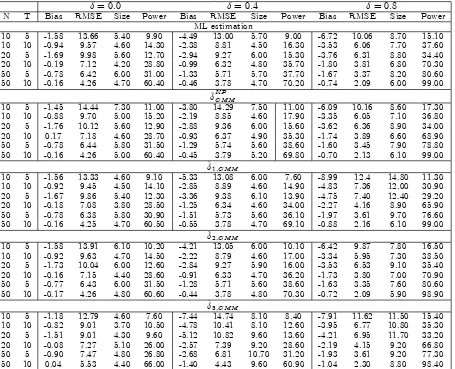
Table 1 shows results for estimators of . For purpose of comparison, we also provide the quasi-ML estimator
of ,^M L. The bias and RMSE of^
KP
GM M decrease asNand/orT get large, for all values of . The size of^
KP GM M
is close to the nominal5%level for = 0:0;0:4, for allN; T larger than10; while it deviates from the 5%level
when T = 5. When = 0:8, the empirical rejection frequencies are slightly larger than the nominal 5%level.
power of^KPGM M. A similar pattern can be observed for the GMM estimator based on other sets of conditions
(i.e.,^1;GM M,^2;GM M and^3;GM M), and for^M L. However, some important di¤erences in the performance of
these estimators can be noted. First,^2;GM M performs overall better than ^
KP
GM M: its bias (in absolute value)
and RMSE are lower than those for^KPGM M, for all values of , and the size is very close to 5%, for = 0:0;0:4.
In the case = 0:8,^2;GM M is slightly oversized whenN andT are small. Notice that results for^2;GM M are
very close to outputs for ^M L in all cases considered. The performance of ^1;GM M and ^3;GM M is similar to
that of^2;GM M when the = 0:0;0:4. For = 0:8,^1;GM M presents some distortions and is characterized by
rejections frequencies larger than5%, ranging between6:10%and14:80%. ^3;GM M has bias and RMSE similar
to^2;GM M, while its size deviates from the5%level. An explanation for this result is that some moments used
in computing^3;GM M might be highly correlated, leading to a nearly-singularQ matrix.
5
Conclusions
We have introduced new moments in a GMM estimation of a spatial regression model. Given that when = 0
some of the suggested moments are redundant, we have proposed to use only a subset of the moments in the estimation procedure. Our Monte Carlo experiments point at conditions (9)-(11) as those that yield the best performance of the GMM estimator.
References
Druska, V. and W. C. Horrace (2004). Generalized moments estimation for spatial panels: indonesian rice farming.
American Journal of Agricultural Economics 86, 185–198.
Fingleton, B. (2008a). A generalized method of moments estimator for a spatial model with moving average errors, with application to real estate prices.Empirical Economics 34, 35 ½U57.
Fingleton, B. (2008b). A generalized method of moments estimator for a spatial panel model with an endogenous spatial lag and spatial moving average errors.Spatial Economic Analysis 3, 27–44.
Kapoor, M., H. H. Kelejian, and I. Prucha (2007). Panel data models with spatially correlated error components.
Journal of Econometrics 140, 97–130.
Kelejian, H. H. and I. Prucha (1999). A generalized moments estimator for the autoregressive parameter in a spatial model.International Economic Review 40, 509–533.
Kelejian, H. H. and I. Prucha (2001). On the asymptotic distribution of the moran i test with applications. Journal of Econometrics 104, 219–257.
Kelejian, H. H. and I. Prucha (2008). Speci…cation and estimation of spatial autoregressive models with autoregressive and heteroskedastic disturbances. Forthcoming, Journal of Econometrics.
Lee, L. F. and X. Liu (2006a). E¢cient GMM estimation of a SAR model with autoregressive disturbances. Mimeo. Lee, L. F. and X. Liu (2006b). E¢cient GMM estimation of high order spatial autoregressive models. Mimeo. Ullah, A. (2004).Finite Sample Econometrics. Oxford: Oxford University Press.
6
Appendix
LetM( ) = [M1( ); :::;Mr( )]0 andMN T( ;^") = [MN T;1( ;^"); :::; MN T;r( ;^")]0, and
R( ;^") =MN T( ;^")0QN T( )MN T( ;^"); Z( ) =M( )0QN T( 0)M( ):
Consistency of the GMM can be showed by proving:
To prove (I), note that
M( ) = '( ) D ; MN T( ;^") =GN T(^")'( ) DgN T(^");
where (here we provide ;'( );D; whenM( )contains (3)-(11), but we recall that our analysis is based on
subsets of these moments)
= 2 6 6 6 6 6 6 6 6 6 6 6 6 6 6 6 6 6 6 4 2E 1 N T PT
t=1u0tSut E N T1 PTt=1utS0Sut 1 0 0 0 0 0 0 0 E N T1 PTt=1u0tS0S2ut E N T1 PTt=1u0tS02S2ut N1T r(S0S) 0 0 0 0 0 0 0
E N T1 PTt=1u0tS0Sut E N T1
PT
t=1u0tS02Sut 0 0 0 0 0 0 0 0
0 0 0 0 1 0 0 0 0 0
0 0 0 0 0 1 0 0 0 0
0 0 0 0 0 0 1 0 0 0
E N T1 PTt=1u0
tSut 0 0 0 0 0 0 1 0 0
E N T1 PTt=1u0tS0S2ut 0 0 0 0 0 0 0 1 0
E N T1 PTt=1u0tS2ut 0 0 0 0 0 0 0 0 1
3 7 7 7 7 7 7 7 7 7 7 7 7 7 7 7 7 7 7 5 ;
'( ) = h 2 2 2
NT r RR
0 2
NT r(R0S0SR)
2
NT r(R0SR)
2
NT r(R)
2
NT r(R0S0S)
2
NT r(R0S)
i0
;
D = I3 I3 I3 0
; =h E N T1 PTt=1u0tut E N T1 PtT=1u0tS0Sut E N T1 PTt=1u0tSut
i0
;
and GN T(^"), gN T(^") are the sample analogues of , . Following Kelejian and Prucha (1999), the proof of
consistency requires the following assumption:
Assumption 5: 0 is non-singular, i.e. its smallest eigenvalue r( 0 )>0.
We have, for k 0k2 K >0,
M( )0QN T( 0)M( ) M( 0)0QN T( 0)M( 0) = ['( ) '( 0)]0 0QN T( 0) ['( ) '( 0)]
r(QN T( 0)) r 0 ['( ) '( 0)]
0
['( ) '( 0)]>0
If moments (6)-(8) alone are included in the analysis, we need to take the following identi…cability conditions:
Assumption 6: '
r( ) 'r( 0)6= 0;for all such thatk 0k2 K >0;andr= 4; :::;9.
To prove (II), let = [GN T(^"); DgN T(^")]andP= [ ; D ], and notice that
R( ;^") Z( ) [ 0Q
N T( ) P0QN T( )P]k'( )k2
p
!0
since, under Assumptions 1-4, and given (16), !p P, and the elements of'( )are bounded.
6.1
The D matrix
D= 2 6 6 6 6 6 6 6 6 6 6 6 6 6 6 4 2 N T PT
t=1^u0tS0^"t 1
2
N T
PT
t=1^u0tS20S^"t N1T r(S0S)
1
N T
PT
t=1^u0tS0S^"t N1^"
0
tS2u^t 0
2
NT r RSRR
0
+RR0S0R0 1
NT r RR
0
2
NT r R
0S0R0S0SR+R0S0SRSR 1
NT r(R
0S0SR)
2
NT r R0S0R0SR+R
0SRSR 1
NT r(R0SR)
1
N T
PT
t=1^u0tS^ut ^
2
NT r(RSR)
1
NT r(R)
1
N T
PT
t=1^u0tS2^ut ^
2
NT r(R0S0R0S)
1
NT r(R0S)
1
N T
PT
t=1^u0tS0S2^ut ^
2
NT r(R
0S0R0S0S) 1
NT r(R
0S0S)
3 7 7 7 7 7 7 7 7 7 7 7 7 7 7 5
Table 1: Small sample properties (X100) of GMM and ML estimates of
= 0:0 = 0:4 = 0:8
N T Bias RMSE Size Power Bias RMSE Size Power Bias RMSE Size Power
ML estimation
10 5 -1.58 13.66 5.40 9.90 -4.49 13.00 5.70 9.00 -6.72 10.06 8.70 15.10
10 10 -0.94 9.57 4.60 14.30 -2.38 8.81 4.50 16.30 -3.53 6.06 7.70 37.60
20 5 -1.69 9.98 5.60 12.70 -2.94 9.27 6.00 15.30 -3.76 6.31 8.80 34.40
20 10 -0.19 7.12 4.20 28.80 -0.99 6.32 4.80 35.70 -1.80 3.81 6.80 70.30
50 5 -0.78 6.42 6.00 31.00 -1.33 5.71 5.70 37.70 -1.67 3.37 8.20 80.60
50 10 -0.16 4.26 4.70 60.40 -0.46 3.78 4.70 70.20 -0.74 2.09 6.00 99.00
^KPGM M
10 5 -1.45 14.44 7.30 11.00 -3.80 14.29 7.50 11.00 -6.09 10.16 8.60 17.30
10 10 -0.88 9.70 5.00 15.20 -2.19 8.85 4.60 17.90 -3.35 6.05 7.10 36.80
20 5 -1.76 10.12 5.60 12.90 -2.88 9.36 6.00 15.60 -3.62 6.36 8.90 34.00
20 10 0.17 7.18 4.60 28.70 -0.93 6.37 4.90 35.30 -1.74 3.89 6.60 68.90
50 5 -0.78 6.44 5.80 31.50 -1.29 5.74 5.60 38.60 -1.60 3.45 7.90 78.80
50 10 -0.16 4.26 5.00 60.40 -0.45 3.79 5.20 69.80 -0.70 2.13 6.10 99.00
^1;GM M
10 5 -1.56 13.33 4.60 9.10 -5.33 13.08 6.00 7.60 -8.99 12.4 14.80 11.30
10 10 -0.92 9.45 4.50 14.10 -2.85 8.89 4.60 14.90 -4.83 7.36 12.00 30.90
20 5 -1.67 9.86 5.40 12.30 -3.36 9.38 6.10 13.90 -4.75 7.40 12.40 29.20
20 10 -0.18 7.08 3.80 28.50 -1.25 6.34 4.60 34.00 -2.27 4.16 8.90 65.90
50 5 -0.78 6.38 5.80 30.90 -1.51 5.73 5.60 36.10 -1.97 3.61 9.70 76.60
50 10 -0.16 4.25 4.70 60.50 -0.55 3.78 4.70 69.10 -0.88 2.16 6.10 99.00
^2;GM M
10 5 -1.58 13.91 6.10 10.20 -4.21 13.05 6.00 10.10 -6.42 9.87 7.80 16.50
10 10 -0.92 9.63 4.70 14.50 -2.22 8.79 4.60 17.00 -3.34 5.95 7.30 38.50
20 5 -1.73 10.04 6.00 12.60 -2.84 9.27 5.90 16.00 -3.53 6.53 9.10 35.40
20 10 -0.16 7.15 4.40 28.60 -0.91 6.33 4.70 36.20 -1.73 3.80 7.00 70.90
50 5 -0.77 6.43 6.00 31.50 -1.28 5.71 5.60 38.60 -1.63 3.35 7.60 80.60
50 10 -0.17 4.26 4.80 60.60 -0.44 3.78 4.80 70.30 -0.72 2.09 5.90 98.90
^3;GM M
10 5 -1.18 12.79 4.60 7.60 -7.44 14.74 8.10 8.40 -7.91 11.62 11.50 15.40
10 10 -0.82 9.01 3.70 10.50 -4.78 10.41 8.10 12.60 -3.95 6.77 10.80 35.30
20 5 -1.51 9.01 4.30 9.60 -5.12 10.82 9.60 13.60 -4.21 6.95 11.70 33.20
20 10 -0.08 7.27 5.10 26.00 -2.57 7.39 9.20 28.60 -2.19 4.15 9.20 66.80
50 5 -0.90 7.47 4.80 26.80 -2.68 6.81 10.70 31.20 -1.93 3.61 9.20 77.30
50 10 0.04 5.53 4.40 66.00 -1.40 4.43 9.60 60.90 -1.04 2.30 8.80 98.40