Munich Personal RePEc Archive
Political Cycles in Active Labor Market
Policies
Mechtel, Mario and Potrafke, Niklas
University of Tuebingen, University of Konstanz
Political Cycles in Active Labor Market Policies
Mario Mechtel
∗and Niklas Potrafke
†‡March 25, 2009
Abstract
This paper examines a framework in which politicians can decrease unemployment via active labor market policies (ALMP). We combine theoretical models on partisan and opportunistic cycles and assume that voters are ignorant of the necessary facts to make informed voting decisions. The model predicts that politicians have incentives for a strategic use of active labor market policies that leads to a political cycle in un-employment and budget deficit. We test the hypotheses predicted by the theoretical model using data from German states from 1985:1 to 2004:11. The results illustrate that opportunistic behavior of politicians can explain the development of ALMP ap-proximated by job-creation schemes.
Keywords: active labor market policies, political cycles, labor market expenditures, opportunistic politicians, partisan politicians
JEL: P16, J08, H72, E62, H61
∗Eberhard Karls University T¨ubingen, Department of Economics, Melanchthonstr. 30, 72074 T¨ubingen, Germany, e-mail: mario.mechtel@uni-tuebingen.de, Phone: + 49 7071 29 78182, Fax: + 49 7071 29 5590.
†University of Konstanz, Department of Economics, Box 138, 78457 Konstanz, Germany, e-mail: niklas.potrafke@uni-konstanz.de, Phone: + 49 7531 88 2137, Fax: + 49 7531 88 3130.
1
Introduction and related literature
This paper introduces a theoretical model that combines aspects of political business cycle theory (PBC) and partisan cycle theory (PT) with the empirical findings that voters do not decide as rationally as often assumed in literature. In our model, politicians face a trade-off between the budget deficit and unemployment, whereas the latter can be fought via active labor market policies (ALMP). The model predicts that opportunistic and partisan motiva-tion of incumbents can explain cycles in ALMP and governmental deficit. Furthermore, we provide empirical evidence from the former West German states during the period 1985:1 to 2004:11 and find that active labor market policies were indeed driven by electoral cycles.
Traditional PBC theory concentrates on politicians facing a short-run Phillips curve trade-off between unemployment and inflation. In such a political setting, as initially devel-oped by Nordhaus (1975) and enhanced by Persson and Tabellini (1990), Rogoff (1990), or Shi and Svensson (2006), political business cycles occur due to incumbents fighting unem-ployment in election years via politically determined positive aggregate demand shocks in order to become re-elected.
Politicians may also have certain ideological beliefs which shape their policies, or they may follow party ideologies. Hibbs (1977) and Alesina (1987) argue that leftist parties attach more importance to unemployment than inflation, while rightwing parties do the exact opposite.
There have been some attempts to combine both bodies of literature, as politicians may plausibly be motivated by both opportunistic and partisan considerations. Frey and Schneider (1978a, 1978b) argue that an incumbent has strong incentives to take opinion polls into account: at times when he is popular, he may implement his favorite partisan politics, whereas he may focus on opportunistic behavior to increase his re-election chances once opinion polls turn sufficiently unfavorable for him. In a recent paper, Sieg (2006) combines rational partisan and opportunistic theory. His model predicts an opportunistic political business cycle with a signalling game in the run-up to an election and a partisan cycle that depends on the winners’ partisan orientation.
During the last decades, literature has uniformly assumed voters to decide in a rational way. We argue that this is unrealistic: empirical evidence suggests that voters are often ignorant of the necessary facts to make informed voting decisions.1Downs (1957) introduced
the theory of rational ignorance as an explanation for the fact that voters often do not know a great deal about relevant topics. When considering a large number of voters, the probability that a particular voter will be the swing-voter is nearly zero. Having the choice between different candidates, voters must be aware of their respective manifestos and many
other criteria such as credibility or institutional framework, in order to identify the monetary consequences of each candidate being elected. Information gathering is costly, as voters may need to watch the news, read newspapers, perhaps buy economics textbooks (to realize the trade-off between unemployment and budget deficit, for example) or consult with experts. It follows that their information costs almost certainly exceed their expected gain in utility from choosing the right candidate. Hence, voters do not have any incentives for information gathering in order to vote rationally in the traditional sense. In a similar vein, Caplan (2001, 2003, 2007) and Caplan and Cowen (2004) argue that voters may be biased in some way and propose to call the voters’ actionsrational irrational voting. Plausible reasons for assuming voters to be biased can be found in the Survey of Americans and Economists on the Economy (Washington Post et al., 1996), which clearly states that voters look at economic problems in a fundamentally different way than economists.
The paper is organized as follows: Section 2 establishes the theoretical model. First, we develop a simple framework for analyzing parties’ optimization problem. Afterwards, we show that due to the different degrees of importance parties attach to unemployment and budget deficit, a cycle will occur. In section 3, empirical evidence from German states is provided. Section 4 concludes the analysis.
2
The Model
2.1
General setting
We assume an economy consisting of an incumbent i, an opponent o, and a fixed number of voters. The incumbent decides on the government’s expenditures in every period t and elections take place in every second period. We assume that the governmental budget is balanced if no active labor market policy is implemented as we want to point out the impor-tance of ALMP. This means that every Euro that is additionally spent for ALMP increases the budget deficit bt ceteris paribus. Without any spending on active labor market policy,
bt = 0 holds.2
The economy’s unemployment rate ut in period t depends on the natural rate of un-employment un and the amount of active labor market policy expenditures. For analytical
simplicity and theoretical clarity, we disregard all other determinants of unemployment, such as overall macroeconomic performance or structural reforms, in order to outline the effects of ALMP and can hence write the unemployment rate in periodtas a function ofun and bt:
ut=un−β·bt (1)
withβ >0.3 Intuitively, the government has the opportunity to decrease the unemployment
rate in every period t via ALMP. The underlying mechanism is simple: the government
2Concerning the interpretation of the results that we are about to derive, one should interpret
btas the
share of budget deficit over GDP. 3For simplicity, we assume
engages in job-creation schemes. On the one hand, the implementation of ALMP increases, ceteris paribus, the budget deficit as ALMP incurs costs and usually does not generate additional revenues.4 On the other hand, unemployment falls, so that the government faces
a clear trade-off between a small governmental deficit and low unemployment.5
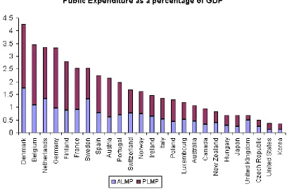
An example of the empirical relevance of this mechanism is Germany, where local and federal governments as well as the Federal Employment Office (Bundesagentur f¨ur Arbeit) have the opportunity to introduce job-creation measures (Arbeitsbeschaffungsmaßnahmen), structural adjustment measures (Strukturanpassungsmaßnahmen), or vocational retraining. Those measures are obviously not free of charge: in Germany, for example, the average monthly cost of a job-creation measure was about 1511 Euro in 2003 (Caliendo and Steiner, 2005). Figure 1 shows that many OECD countries (particularly European ones) face ALMP expenditures close to one percent of GDP (OECD, 2007, p. 231), which represents a con-siderable fraction of freely disposable government expenditure.
Figure 1 about here
Official German unemployment statistics do not include people engaged in ALMP mea-sures (Bundesagentur fuer Arbeit, 2004). Hence German politicians face exactly the same trade-off as stated in our model.
To decide whether to fully inform oneself about political and economic relationships or not, each voter compares his expected gain in utility from selecting the right candidate with the costs of gathering information. Whenever these costs outweigh the expected gain in utility, a voter does not engage in collecting information at all. Each voter’s expected net gain in utility (NGU) from choosing the right candidate in an election involving two candidates can be stated as
NGU =ρ·[payoffright−payoffwrong]−information costs,
where payoffkis the present value of the payoff resulting from candidatek’s,k = right,wrong, future policies, e.g. tax reforms or similar things. ρis the probability of each voter being the swing voter. One can easily see that the expected gain in utility from supporting the right candidate will be extremely low in an economy with a reasonable large number of voters,
β. In reality, one could interpret β as a policy variable in the sense of politicians’ ability to create new and heterogenous ALMP measures at a lower price. This would mean an increase in β: The decrease in unemployment is higher for a given amount ofbt. An example of a politically induced increase inβ could be
the 1-Euro jobs in Germany, which allow politicians to decrease unemployment whilst paying a lower price, measured as the variation in budget deficit.
4Even if a job-creation measure generated additional revenues, these would certainly not exceed the expenditure required to create the measure. Hence,btincreases.
5Note, however, that ALMP in period
even if both parties differ greatly in their fiscal consequences. Therefore, it is extremely unlikely that the net gain in utility is positive. Hence, rational voters have no incentive to inform themselves about political as well as economic relationships.6
Although voters have no incentives to actively look for information, we assume that they somehow become informed about the economic performance.7 We choose the unemployment
rate as a proxy for the economic performance as unemployment is a major concern in almost every industrialized country. In the overwhelming majority of pre-election surveys voters report unemployment as the greatest problem in their society.8
Furthermore, as recent research shows, the self-interested voter hypothesis fails in empir-ical tests.9 Hence, our assumption of voters looking implicitly at a macro variable such as
unemployment is similar to what is called sociotropic voting. In our model, voters are not concerned with the consequences for their own wallets, but actually vote for politicians who they suppose to be good for the country.
Formally, we assume the voting behavior of each voter to depend on the current unem-ployment rate ut and a random variable µt that is distributed in the interval [−z; +z] and
E(µ) = 0. µt can be interpreted as voters or informational bias (see Caplan and Cowen, 2004, for a discussion) as well as the expressive voting hypothesis established by Brennan and Lomasky (1993). Within the model,µtbasically ensures that incumbents are not able to guarantee their re-election. We assume that voters are identical. Therefore, the probability of an incumbent of partyi being re-elected can thus be written as
p=p(ut(bt), µt). (2)
We assume that p is distributed in the interval (0,1) with ∂u∂pt < 0 (and hence ∂b∂pt > 0), but that the incumbent is not able to set a sufficiently low unemployment rate to make his re-election a certain event.10 The structure of the voting probability implicitly assumes that voters have a short memory. Case studies concerning very volatile popularity data for the leading politicians support this assumption (see, for example, Forschungsgruppe Wahlen, 2008). Note, however, that the voting probability can be written as in (2) because rational voters do not have an incentive to inform themselves about political and economic relation-ships or mechanisms. Although they are unaware of economic mechanisms and interrelations,
6For discussion on the topic see Downs (1957), Caplan (2001, 2003, 2007), as well as Jones and Dawson (2008).
7This is in line with e.g. Downs (1957). It would be inappropriate to assume that voters do not receive any information about the economic performance at all. Imagine voters watching TV or passing a newsstand in the street - they certainly get some kind of information about their country’s economic performance despite not actively searching for information.
8According to infratest dimap (2005), 88 percent of the voters mentioned “unemployment” when asked what (in their opinion) the most important political problems were on the day of the German Bundestagswahl in 2005. Although multiple answers were possible, only 5 percent mentioned “public debt”.
9
See Caplan, 2002 for a discussion of this topic. 10
they have some knowledge about macroeconomic performance, here measured by unemploy-ment. Therefore, our analysis differs from other recent models on political or partisan cycles in assuming that voters do not actively search for information and may be biased in some way.
Politicians maximize their expected utility, which consists of two elements. On the one hand, an ideologically motivated outcome component including unemployment and budget deficits. On the other hand, an ego rent r > 0 is generated by holding office. This means that we combine two essential elements of political business cycle literature: as stated by Nordhaus (1975), Rogoff (1990), and Persson and Tabellini (1990), the political optimization problem has an opportunistic component insofar as politicians prefer to be in office rather than not. However, following Hibbs (1977) and Alesina (1987), politicians also face a trade-off between two bads.
In our model, elections take place in every second period. Therefore, the timing of the two period model is as follows: at the beginning of periodt, the incumbent sets his favored unemployment rate using ALMP. Afterwards, voters decide who they want in office for the next two periods: either the incumbent i who is a member of the left (L) or the right (R) party, or the opponent who is a member of the other party. Int+ 1, the winner implements his favorite policy.
The expected utility of incumbent i can therefore be written as
E(Vi) = θi·
−αi(ui
t)2−(b i
t)2 + (1−θ i)ri
t
+p(ut(bt), µt)·δi·
θi·
−αi(ui
t+1)2−(bit+1)2 + (1−θi)rti+1
+ (1−p(ut(bt), µt))·δi·θi
−αi(uot+1)2 −(b
o
t+1)2 ,
(3)
where δi denotes the discount rate which we assume to be the same for all candidates of
party L, respectively R. ri
t is the candidate’s ego rent from holding office. uot+1 and bot+1
(ui
t+1 and bit+1) denote the values of unemployment and the budget deficit in period t+ 1
that would result if the opponent (incumbent) won the election. Incumbent i’s relative preference of ut to bt is measured by αi. θi is an exogenous parameter that measures the
importance of ideologic goals relative to the ego rent ri
t.11 Over time, however, θi may
differ between different incumbents of the same party. The politicians’ utility decreases with unemployment and the budget deficit at an increasing rate (∂2E∂u(V2i)
t < 0 and
∂2E(Vi
)
∂b2
t < 0).
The latter implicates the existence of something such as an implicit intertemporal budget constraint.12
11
One could also imagineθi
to be endogenous, depending on election polls for example, which would be an application of the idea developed by Frey and Schneider (1978).
12
The two parties have preferences concerning the unemployment rate and the budget deficit. The borderline case αL =αR could be interpreted as a purely opportunistic version
of our model. We assume αL > αR to hold.13 For a given budget deficit, an incumbent
of the leftist party dislikes unemployment more than a rightwing incumbent does. For simplicity and analytical convenience, we supposerL
t =rRt =rtL+1 =rtR+1 =r to hold, which
seems plausible as, for example, salary payments to the incumbent do not depend on the incumbent’s partisan orientation.
2.2
Non-election periods
To solve the model, we first consider what happens in the non-election periodt+ 1. As there are no elections, politicians can neglect their influence onp because there simply is none.
Therefore, the incumbentiwill maximize his periodt+1 utility, taking all future decisions as exogenously given and taking the trade-off between unemployment and budget deficit (1) into account.
We can rewrite the incumbent’s maximization problem as
max bt+1
θi·
−αiu2
t+1−(bt+1)2 + (1−θi)r s.t. ut+1 =un−β·bt+1.
Using the first order condition, the optimal budget deficit in the non-election period t+ 1 for incumbent i turns out to be
bi∗
t+1 =
αiβun
1 +αiβ2. (4)
We can easily see that ∂b
i∗ t+1
∂un > 0 holds: the optimal budget deficit for an incumbent of
type i increases with the natural rate of unemployment. Note that bi∗
t+1 does not depend
onθi because no elections take place and, therefore, there is no need to weigh the ideologic
against the opportunistic goal.
The optimal budget deficit in t+ 1 varies positively withαi:
∂bi∗
t+1
∂αi =
βun
(1 +αiβ2)2 >0
since we assumedβ >0. Hence, assumingαr < αl, we can conclude that the optimal budget
deficit in a non-election period is higher if the leftist party is the incumbent. Using (4), we can determine ui∗
t+1:
ui∗
t+1 =un−
αiβ2un
1 +αiβ2 (5)
where ∂u
i∗ t+1
∂αi <0 holds, which means that the optimal period t+ 1 unemployment rate from
the incumbent’s point of view is lower for the leftwing party. However, ui∗
t+1 also does not
depend onθi.
The analysis above clearly shows that in our model there will be political determined differences in b and u in all periods without an election. Whenever a leftist politician is in power, unemployment will be lower at the expense of a higher budget deficit. Therefore, in non-election periods there will be fluctuations in ALMP and unemployment, depending on the incumbent’s partisan orientation.
2.3
Election periods
Given the politicians’ non election year strategies described in (4), we can calculate their policy choices in election periods using (3). Incumbent i’s optimization problem is
max bt
E(Vi) =θi·
−αi(un−βbt)2−b2t + (1−θ i
)r
+p(ut(bt), µt)·δ·hθi·n−αi· un−βbi∗
t+1
2
− bi∗
t+1
2o
+ (1−θi)ri
+ (1−p(ut(bt), µt))·δ·hθi·n−αi· un−βbo∗
t+1
2
− bo∗
t+1
2oi
,
(6)
where o is the candidate of the other party.
Using the respective first order condition as well as (4), the incumbent i’s optimal budget deficit in t amounts to
bi∗
t =
αiβun
1 +αiβ2
+ ∂p
∂ut ∂ut
∂bt ·
δ
2(1 +αiβ2) ·
"
−αi
un− α iβ2un
1 +αiβ2
2
−
αiβun
1 +αiβ2
2
+ (1−θ
i)r θi # − ∂p ∂ut ∂ut ∂bt · δ
2(1 +αiβ2) ·
"
−αi
un− α
oβ2un
1 +αoβ2
2
−
αoβun
1 +αoβ2
2#
.
(7)
In order to determine whether there will be an opportunistic cycle component, we com-pare bt with bt+1. As the first term of (7) equals incumbent i’s optimal budget deficit in
t+ 1, we have to take a look at the second and third term of (7). For completely identical politicians, which means αR =αL, we can clearly see that the budget deficit in an election
Under more general conditions than in the last paragraph,bt> bt+1 holds whenever
−αi·
un− α
iβ2un
1 +αiβ2
2
−
αiβun
1 +αiβ2
2
+(1−θ
i)r θi >
−αi·
un− α oβ2un
1 +αoβ
2
−
αoβun
1 +αoβ2
2 (8)
is fulfilled.
Proposition: bi∗
t > bit∗+1 holds for all i=L, R as long as r ≥0.
Proof: Using (8) and rearranging terms yields:
r >− β
2(un)2(αi−αo)2
(1 +αiβ2)(1 +αoβ2)2
θi
(1−θi) <0. (9)
Hence, we conclude that ALMP expenditures in election years exceed ALMP in non-election years even if we assumed that there was no ego rent from holding office because there is an ideological benefit from holding office.14 For a positive r,bt would even be higher, the higher
r is.
As incumbents seek re-election, they always face an incentive to lower unemployment figures in election periods as long as r≥0, which leads to an increase of the budget deficit. There is only one imaginable situation where bt > bt+1 does not hold. This is the case for
identical politicians (αL = αR) who do not benefit from being incumbent (r = 0), which
does not seem to be realistic at all.
Hence, using (7) and (1), we can conclude that ui∗
t < uit∗+1 holds for i = L, R as the
election period budget deficit exceeds the budget deficit in a non-election period for both types of parties.
Finally, we can determine the effect of a change in θi on bi∗
t and uit∗. Differentiation of
(7) with respect to θi obtains
∂bi∗
t ∂θi∗ =−
∂p ∂ut
∂ut ∂bt
δr
1 +αiβ2
1−θi
2θi2 +
1 2θi
<0.
If the relative importance the incumbentiattaches to his partisan goals increases, the budget deficit intdecreases because the re-election goal loses importance. Therefore, ∂uit∗
∂θi∗ >0 holds.
Hence, in our model a political business cycle occurs due to systematic deviations in active labor market policies which depend on the incumbent’s partisan orientation and on the timing of the election. A crucial assumption is the voters’ behavior. For them, it is fully rational not to gather any information about political and economic backgrounds and interrelations. However, they do receive some information about the macroeconomic performance. If voters were rational in the traditional sense, politicians would not necessarily
14Note that (9) reveals that even for a negative
r (e.g. being interpreted as a burden of responsibility),
bi∗ t > b
i∗
be able to gain from expanding the public deficit in election periods as the fully informed voters would be aware of the underlying trade-off between unemployment and public debt. Yet empirical evidence suggests that people are not fully rational, and therefore our portrait seems to be appropriate.
3
Empirical analysis
3.1
Institutional background
3.1.1 Active labor market policies in Germany
The so-called active labor market policy is concerned with reintegration of unemployed persons into the labor market by, for example, subsidising wages or by means of job creation schemes.15 These ALMP programs, in Germany supervised by the Federal Employment
Agency (Bundesagentur f¨ur Arbeit, FEA) are intended to help overcome the unemployment problem. Historically, the ALMP programs were one of the most important innovations of the Job Promotion Act (AFG, Arbeitsfoerderungsgesetz), which formed the legal basis for labor market policies in Germany in the period 1969 to 1997. In 1998, the Social Code (Sozialgesetzbuch, SGB) III was adopted and it was intended that ALMP should become further intensified.
ALMP does not only play a role at the federal level, however.16 In practice, it is not
only the FEA that implements ALMP, but above all, the Laender Employment Agencies (Landesanstalten, LEA) as Germany is a federal state (for further details on labor market policies in Germany and the institutional set-up of job creation schemes see e.g. Thomsen, 2007, p. 16).
In fact, the states’ governments can implement their preferred labor market policies not only by subsidizing particular ALMPs with money from their own budgets, but also by setting administrative guidelines within the LEAs. There is an intense interaction, or even sleaze between the political decision makers and leading civil servants in the LEAs.17 Besides
the programmes initiated by the LEAs and the local agencies, each state government can
15There are several ALMP instruments which broadly remained the same but were extended over time. Thomsen (2007) refers to the SGB III as a legal basis and distinguishes between “Measures to Enhance and Adjust the Qualification of the Individuals”, “Counselling and Assistance for Regional and Vocational Mobility” and “Subsidised Employment”. The latter category consists of wage subsidies and two groups of employment programs, namely job creation schemes and structural adjustment schemes. They both establish the so-called second labor market.
16Some anecdotic evidence concerning the relevance of job-creation schemes in the run-up to an election can be found in the elections for the Bundestag in 1994 and 1998. The then-chancellor Helmut Kohl used ALMP measures to fight unemployment to a notable extent.
implement additional ALMP measures. Therefore, the trade-off between unemployment and budget deficit applied in our theoretical model directly appears in reality: for any given level of local or LEA activity, a States’ government can implement additional ALMP measures.
At the beginning of the 1980s, some German states first introduced their own programs on employment promotion18, such as a special program of the senate in Hamburg in October
1982.19 Throughout the period of the European structural fund of 1988, ALMP programs
and activities of the German states generally increased. However, activities and intensity varied between the states. For example, the Saarland heavily relied on ALMP programs in their labor market policies. Even today, the state’s government explicitly highlights its activities with respect to ALMP.
Another example for the role of government in ALMP measures is the state North Rhine-Westphalia. After the Rhine flood at the beginning of 1995, unemployed persons were assigned to job-creation schemes to assist in the flood plain and thus no longer appeared in official unemployment statistics. Thus after the flood, unemployment had also declined, just in time for the 1995 election of the state parliament. Another recent example is Hesse in 2008. As a precondition to joining a coalition with Social Democrats and Greens, the socialist party “Die Linke” demanded job-creation schemes for 25.000 people.20
However, ALMP programs already started in the beginning of the 1980s in the former western states, so our analysis will focus on this group of 10 states. In particular, we will examine job-creation schemes until 2004.21 On the one hand, this is due to the fact that
job-creation schemes were an prominent policy instrument and they became less important since the end of 2004. On the other hand, job-creation schemes are the ALMP measure with the best and most comparable data supply in Germany.
3.1.2 Parties, government coalitions, legislative periods and elections
There are two large parties in Germany, the leftist Social Democratic Party (SPD) and the conservative Christian Democratic Union (CDU). In Bavaria, Germany’s federal state with the largest area, the conservatives are not represented by the CDU but by their sister party, the Christian Social Party (CSU). However, there is no party competition between them and they form a single faction in the federal parliament (Bundestag). That is why we label both CDU in the following empirical analysis. All federal chancellors and state prime ministers were members of one of these two big blocks, SPD and CDU. Therefore, one can test for partisan effects simply on this left-right dimension.
Nevertheless, the much smaller Free Democratic Party (FDP) and Green party (GR) have played an important role as coalition partners in the former Western states. While the
18For a brief overview, see Kohler (2004: p. 50).
19The program first amounted to 51 million Euro and was later enhanced, see Hombach (1984, p.190). 20http://www.spiegel.de/politik/deutschland/0,1518,574355,00.html.
SPD has formed coalitions with all the other three parties, the CDU never formed a coalition with the Greens on the federal or state level during the period analyzed in this paper. We will also consider the impacts of the different coalition types, because it is possible that the simple leftwing-rightwing dimension may neglect ideological differences between government parties within a ”camp” (e.g. for the Left between SPD/FDP and SPD/GR coalitions). As minority governments and other government formations have played a negligible role, they will be subsumed under the coalition types mentioned above. There are no fixed election dates across the German states and the legislative periods last between four and five years. However, early elections may be called independently. So far, less than ten percent of the elections in the German states were early elections.
3.2
Data and empirical strategy
3.2.1 Data and variables
The data set contains monthly data for the number of job-creation schemes in the period 1985:1 to 2004:11 (levels) for the ten former West German states. These data are provided by Germany’s Federal Employment Office. We do not include the former East German states and also do not consider Berlin because it was divided before the German unification and therefore the data contain structural breaks.
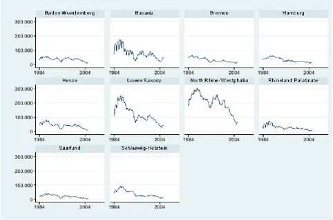
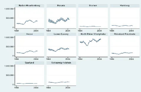
Figures 2 and 3 illustrate the change in the number of job-creation schemes and the number of unemployed persons. The development of the job-creation schemes and unem-ployment are subject to a seasonal pattern. Unemunem-ployment is higher in winter than in sum-mer, whereas the cyclical pattern of the job-creation schemes is time-delayed. Furthermore, there are differences in time and between the single states. For example, unemployment as well as the number of job-creation schemes decreased at the end of the 1980s and reached their minima after the German unification in 1990. Subsequently, both increased steadily in almost every German state. Overall, we control for these effects using fixed year, monthly and state dummies in the econometric model.
Figures 2 and 3 about here
3.2.2 The empirical model
The basic econometric panel data model has the following appearance: ∆ln job-creation schemesiym=X
j
αj Political variableijym
+λm+γy+ηi+uiym
(10)
with i= 1, ...,10;j = 1, ...,6;m= 1, ...,12;y= 1985, ...,2004.
The dependent variable ∆ln job-creation schemesiym denotes the growth rate in the
num-ber of job-creation schemes in every single state.22 Panel unit root tests show that this
variable is stationary. The appendix provides comments on the chosen test procedures. Moreover, λm describes fixed monthly, γy fixed year23, and ηi fixed state effects.24
P
jαj Political variableijym describes the political variables on which this study focuses.
First, the variable Election(12) takes the timing of the elections into account. It takes on the value of one in the twelve months before an election. In all other months, its values are set at zero. Therefore, we directly control for fluctuations and the fact that there are no fixed election dates in Germany. We will use this electoral variable as a benchmark. For robustness checks, we also apply different codings such as ten, eight, six, and four months before the elections.
We test the differences between leftist and rightwing governments predicted by our model on the simple leftwing-rightwing scale using the variable “Left” and different coalition type dummies, separately. The dummy “Left” takes on the value of one in periods when an SPD Prime Minister was in office (excluding grand coalitions) and zero otherwise. In the alterna-tive specification, the coalition type dummies take on the value of one when the considered coalition type was in power and zero otherwise. We distinguish between six different coalition types that governed in the former Western German states: CDU, CDU/FDP, CDU/SPD, SPD/FDP, SPD/GR, and SPD. With respect to the grand coalitions, we do not distinguish which of the two parties appointed the Prime Minister. To avoid multicollinearity between these dummies, one of them must function as the reference category (here SPD). The esti-mated effects of the other dummies must then be interpreted as deviations from this reference category. Descriptive statistics are provided in Table 1.
Table 1 about here
The basic model is estimated by feasible generalized least squares in a common fixed effects framework initially. In addition, we apply heteroskedastic and autocorrelation con-sistent (HAC) Newey-West type (Newey and West, 1987) standard errors and variance-covariance estimates, because the Wooldridge test (Wooldridge, 2002, p. 176-177) for serial
22
We use the number of job-creation schemes instead of the inflows into job-creation schemes as the measures vary in duration.
23Note that this also fixes specific historical events like the German unification.
correlation in the idiosyncratic errors of a linear panel-data model implies the existence of strong arbitrary serial correlation. Moreover, the number of job creation schemes is directly related to the number of unemployed persons. Therefore, we include the lagged number of unemployed persons in a further step as job-creation schemes are used in reaction to high unemployment. We address the persistency and remaining seasonality of the dependent variable and the time-delayed interaction of unemployed persons and job-creation schemes by including a battery of lagged dependent variables and lags of the unemployed persons variable.
3.3
Estimation results
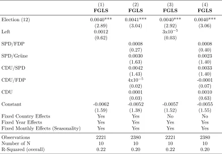
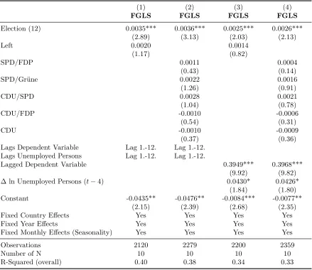
Table 2 shows the regression results of the initial fixed (columns 1 and 2) and random effects (columns 3 and 4) regressions with heteroskedastic and autocorrelation consistent (HAC) Newey-West type standard errors. We cannot reject the Hausman-Test in favor of the random effects model. However, the regression results of the fixed and random effects differ only slightly. Table 2 provides the coefficients and t-ratios (absolute values) for every single equation.
Table 2 about here
In accordance with our theoretical model, politicians increased the number of job-creation schemes in election years. The coefficient tells us that before elections in the German states, the growth rate of the job-creation schemes increased by about 0.4 percent per month. Thus, politicians behaved opportunistically to become re-elected. Moreover, the results do not support the hypothesis that leftist governments implemented more active labor market policies than rightwing governments. The coefficients do have the expected signs but are statistically insignificant. On the one hand, this result could be interpreted as being due to small ideological differences between the parties. Within our model, one might argue that there was only a small difference between αL and αR, if there was one at all. On the
other hand, one might argue that politicians did not care much about political outcomes and concentrated on staying in office. This could be seen as a reference to a small θL and θR within our model.
Table 3 about here
an elasticity of about 0.4. The impact of the four months lagged number of unemployment persons is statistically significant on a 10 percent level and the coefficient reveals that when the lagged number of unemployed persons increased by one percent, the number of job-creation schemes increased by approximately 0.04 percent. In any case, the inclusion of the lagged dependent variables and the lagged number of unemployed persons does not affect our inferences regarding the political variables at all. Again, the estimation results provide evidence for an electoral cycle. The point estimate of the Election(12) only slightly decreases and thus implies that before elections in the German states, the growth rate of the job-creation schemes increased by about 0.3 percent.
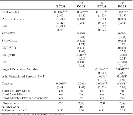
Table 4 and 5 about here
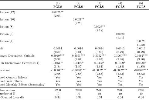
We tested further specifications including the different election-year variables and cod-ings described above and results did not change. Table 4 reports the regression results when a post-election(12) variable is included. This variable takes on the value of one in the twelve months after an election and is zero otherwise. In line with our theoretical predictions, the post-election variable is statistically insignificant across the specifications while the elec-tion(12) variable remains statistically significant and the numerical impact does not change. Table 5 shows the regression results when the election variable takes on the value one in the ten, eight, six or four months before the election (and zero otherwise). The results sug-gest that incumbents did not increase job-creation schemes directly before elections as the election(6) and election(4) variable turn to be statistically insignificant. This finding is also in line with theoretical and intuitive predictions of political opportunism because it simply takes some time to implement these job-creation schemes and opportunistic politicians would not implement these measures if they could not get re-elected due to their activities.
Moreover, we checked for the sensitivity of the results to individual states. To rule out this possibility, we performed the regressions again, excluding one state at a time. Overall, the inferences are robust in that they are not subject to the inclusion of particular countries. However, the impact of the election variables declines when Schleswig-Holstein and the Saarland are excluded, yet remains significant on the 5 percent level.
In addition, we aggregated our monthly to yearly data and run the regressions with annual data. These regression results perfectly correspond with our inferences using monthly data: We find evidence for electoral cycles, whereas the partisan variables have the expected signs but remain statistically insignificant.
4
Conclusion
literature claims voters to be sociotropic. As opinion polls reveal that unemployment is the most - or at least one of the most - important political topics in nearly all industrialized countries, we use unemployment as the sociotropic factor in our model. Second, electoral outcome depends on a factor which can be interpreted as a voter bias, according to Caplan and Cowen (2004) as well as the expressive voting hypothesis established by Brennan and Lomasky (1993).
We find that politically motivated cycles, with respect to budget deficits and unemploy-ment, do occur. Before an election takes place, politicians have the incentive to lower the unemployment rates by using active labor market policy measures. After the election, the (new) incumbent enforces the kind of ALMP that maximizes his utility. Post election cycles in both variables occur due to partisan differences between politicians.
5
Appendix
Variable Obs. Mean Std. Dev. Min Max Source
Job Creation Schemes 2390 6326.23 6440.11 172 30711 Federal Employment Agency Unemployed Persons 2390 231364.50 211696.90 33679 921330 Federal Employment Agency
Election (12) 2390 0.24 0.43 0 1 Potrafke (2006)
Left 2231 0.62 0.49 0 1 Potrafke (2006)
SPD 2390 0.34 0.47 0 1 Potrafke (2006)
SPD/FDP 2390 0.11 0.31 0 1 Potrafke (2006)
SPD/GR 2390 0.13 0.34 0 1 Potrafke (2006)
CDU/SPD 2390 0.07 0.25 0 1 Potrafke (2006)
CDU/FDP 2390 0.15 0.36 0 1 Potrafke (2006)
CDU 2390 0.20 0.40 0 1 Potrafke (2006)
[image:21.595.58.574.81.225.2]Notes: Absolute value of t-statistics in brackets, * significant at 10%, ** significant at 5%, *** significant at 1%
(1) (2) (3) (4)
FGLS FGLS FGLS FGLS
Election (12) 0.0040*** 0.0041*** 0.0040*** 0.0040*** (2.89) (3.04) (2.92) (3.06)
Left 0.0012 3x10⁻⁵
(0.62) (0.03)
SPD/FDP 0.0008 0.0008
(0.27) (0.40)
SPD/Gr¨une 0.0030 0.0023
(1.63) (1.40)
CDU/SPD 0.0042 0.0033
(1.43) (1.40)
CDU/FDP 4x10⁻⁵ -0.0001
(0.02) (0.07)
CDU 0.0001 0.0010
(0.03) (0.63)
Constant -0.0062 -0.0052 -0.0057 -0.0055
(1.59) (1.38) (1.52) (1.55)
Fixed Country Effects Yes Yes No No
Fixed Year Effects Yes Yes Yes Yes
Fixed Monthly Effects (Seasonality) Yes Yes Yes Yes
Observations 2221 2380 2221 2380
Number of N 10 10 10 10
R-Squared (overall) 0.22 0.20 0.22 0.20
Notes: Absolute value of t-statistics in brackets
[image:22.595.73.513.188.493.2]* significant at 10%, ** significant at 5%, *** significant at 1%
(1) (2) (3) (4)
FGLS FGLS FGLS FGLS
Election (12) 0.0035*** 0.0036*** 0.0025*** 0.0026*** (2.89) (3.13) (2.03) (2.13)
Left 0.0020 0.0014
(1.17) (0.82)
SPD/FDP 0.0011 0.0004
(0.43) (0.14)
SPD/Gr¨une 0.0022 0.0016
(1.26) (0.91)
CDU/SPD 0.0028 0.0021
(1.04) (0.78)
CDU/FDP -0.0010 -0.0006
(0.54) (0.31)
CDU -0.0010 -0.0009
(0.37) (0.36)
Lags Dependent Variable Lag 1.-12. Lag 1.-12. Lags Unemployed Persons Lag 1.-12. Lag 1.-12.
Lagged Dependent Variable 0.3949*** 0.3968*** (9.92) (9.82) ∆ ln Unemployed Persons (t−4) 0.0430* 0.0426*
(1.84) (1.80) Constant -0.0435** -0.0476** -0.0084*** -0.0077**
(2.15) (2.39) (2.68) (2.35)
Fixed Country Effects Yes Yes Yes Yes
Fixed Year Effects Yes Yes Yes Yes
Fixed Monthly Effects (Seasonality) Yes Yes Yes Yes
Observations 2120 2279 2200 2359
Number of N 10 10 10 10
R-Squared (overall) 0.40 0.38 0.34 0.33
Notes: Absolute value of t-statistics in brackets
[image:23.595.75.514.151.531.2]* significant at 10%, ** significant at 5%, *** significant at 1%
(1) (2) (3) (4)
FGLS FGLS FGLS FGLS
Election (12) 0.0045*** 0.0043*** 0.0029** 0.0027** (3.07) (3.02) (2.20) (2.14) Post-Election (12) 0.0016 0.0007 0.0011 0.0005 (1.27) (0.54) (0.96) (0.43)
Left 0.0013 0.0015
(0.68) (0.87)
SPD/FDP 0.0008 0.0004
(0.26) (0.13)
SPD/Gr¨une 0.0030 0.0016
(1.63) (0.92)
CDU/SPD 0.0041 0.0020
(1.40) (0.75)
CDU/FDP 3x10⁻⁵ -0.0006
(0.01) (0.34)
CDU 0.0001 -0.0009
(0.02) (0.37)
Lagged Dependent Variable 0.3944*** 0.3967*** (9.91) (9.81) ∆ ln Unemployed Persons (t−4) 0.0434* 0.0428*
(1.85) (1.80) Constant -0.0065* -0.0053 -0.0087*** -0.0078**
(1.67) (1.40) (2.76) (2.35)
Fixed Country Effects Yes Yes Yes Yes
Fixed Year Effects Yes Yes Yes Yes
Fixed Monthly Effects (Seasonality) Yes Yes Yes Yes
Observations 2221 2380 2200 2359
Number of N 10 10 10 10
R-Squared (overall) 0.22 0.20 0.34 0.33
Notes: Absolute value of t-statistics in brackets
[image:24.595.70.515.145.529.2]* significant at 10%, ** significant at 5%, *** significant at 1%
(1) (2) (3) (4) (5)
FGLS FGLS FGLS FGLS FGLS
Election (12) 0.0025** (2.03)
Election (10) 0.0027**
(2.29)
Election (8) 0.0027**
(2.18)
Election (6) 0.0020
(1.41)
Election (4) 0.0023
(1.62)
Left 0.0014 0.0014 0.0014 0.0013 0.0013
(0.82) (0.81) (0.80) (0.79) (0.79) Lagged Dependent Variable 0.3949*** 0.3951*** 0.3952*** 0.3960*** 0.3962***
(9.92) (9.87) (9.87) (9.88) (9.90) ∆ ln Unemployed Persons (t-4) 0.0430* 0.0429* 0.0428* 0.0429* 0.0430*
(1.84) (1.85) (1.84) (1.85) (1.85) Constant -0.0084*** -0.0083*** -0.0082*** -0.0082*** -0.0082***
(2.68) (2.68) (2.63) (2.63) (2.63)
Fixed Country Effects Yes Yes Yes Yes Yes
Fixed Year Effects Yes Yes Yes Yes Yes
Fixed Monthly Effects (Seasonality) Yes Yes Yes Yes Yes
Observations 2200 2200 2200 2200 2200
Number of N 10 10 10 10 10
R-Squared (overall) 0.34 0.34 0.34 0.34 0.34
[image:25.595.71.562.175.505.2]Notes: Absolute value of t-statistics in brackets. * significant at 10%, ** significant at 5%, *** significant at 1%
5.1
Panel unit root tests
In order to test the stationarity of the time series, we applied the following panel unit root tests by: Levin, Lin and Chu (2002); Im, Pesaran and Shin (2003) and the Fisher tests with reference to Maddala and Wu (1999) and Choi (2001). Breitung and Pesaran (2008) provide a detailed description of the recent panel unit root tests. The results were obtained using Eviews 6.0. In comparison to STATA 9.1, Eviews 6.0 allows the application of the respective tests on unbalanced panels, it considers an automatic lag length selection through the use of Information Criteria and also contains the Breitung (2000) test. Regarding the first three tests, maximum lag lengths are automatically selected based on the Schwarz Information Criterion. The remaining two tests use the Bartlett kernel for the Newey-West bandwidth selection. The probabilities for the Fisher tests are computed using an asymptotic Chi-square distribution. All other tests assume asymptotic normality.
The test results indicate that the growth rates of the job-creation schemes and the number of unemployed persons are stationary.
References
[1] Alesina, A. (1987). ’Macroeconomic Policy in a Two-Party System as a Repeated Game’,
The Quarterly Journal of Economics, vol. 102(3), pp. 651-678.
[2] Alesina, A., Roubini, N. and Cohen, G.D. (1997).Political cycles and the macroeconomy, Cambridge, Massachusetts: MIT Press.
[3] Breitung, J. (2000). ’The local power of some unit root tests for panel data’, in Baltagi, B. (eds.),Advances in Econometrics, Vol. 15: Nonstationary panels, panel cointegration, and dynamic panels, pp. 161-178, Amsterdam: JAI Press.
[4] Breitung, J. and Pesaran, M.H. (2008). ’Unit Roots and cointegration in panels’, in Matyas, L. and Sevestre, P. (eds), The econometrics of panel data: fundamentals and recent developments in theory and practice, pp. 279-322, Dordrecht: Kluwer Academic Publishers.
[5] Brennan, G. and Lomasky, L. (1993). Democracy and Decision: The Pure Theory of Electoral Preference, Cambridge: Cambridge University Press.
[6] Bundesagentur f¨ur Arbeit (2004).Begriff der Arbeitslosigkeit in der Statistik unter SGB II und SGB III.
[7] Bundesagentur f¨ur Arbeit (2007). Data on employment, unemployment, and ALMP.
[8] Caliendo, M. and Steiner, V. (2005). ’Aktive Arbeitsmarktpolitik in Deutschland. Be-standsaufnahme und Bewertung der mikro¨okonomischen Evaluationsergebnisse’, DIW Discussion Papers, 515.
[9] Caplan, B. (2001). ’Rational ignorance versus rational irrationality’,Kyklos, vol. 54, pp. 3-26.
[10] Caplan, B. (2002). ’Sociotropes, Systematic Bias, and Political Failure: Reflections on the Survey of Americans and Economists on the Economy’, Social Science Quarterly, vol. 83(2), pp. 416-435.
[11] Caplan, B. (2003). ’The Logic of Collective Belief’, Rationality and Society, vol. 15(2), pp. 218-42.
[12] Caplan, B. and Cowen, T. (2004). ’Do we underestimate the benefits of cultural com-petition?’, The American Economic Review, vol. 94(2), pp. 402-407.
[14] Choi, I. (2001). ’Unit root tests for panel data’, Journal of International Money and Finance, vol. 20(2), pp. 249-272.
[15] Downs, A. (1957).An Economic Theory of Democracy, New York: Harper.
[16] Forschungsgruppe Wahlen (2008). Politbarometer 1977 bis 2005 auf CD-ROM,
http://www.gesis.org/Datenservice/Politbarometer/index.htm.
[17] Frey, B.S. and Schneider, F. (1978a). ’An Empirical Study of Politico-Economic Inter-action in the United States’, The Review of Economics and Statistics, vol. 60(2), pp. 174-183.
[18] Frey, B.S. and Schneider, F. (1978b). ’A politic-economic model of the United Kingdom’,
The Economic Journal, vol. 88, pp. 243-253.
[19] Gerfin, M. and Lechner, M. (2002). ’A Microeconometric Evaluation Of The Active Labour Market Policy In Switzerland’, The Economic Journal, vol. 112, pp. 854-893.
[20] Hagen, T. and Steiner, V. (2000). Von der Finanzierung der Arbeitslosigkeit zur F¨orderung von Arbeit, Baden-Baden.
[21] Hibbs, D.A. (1977). ’Political Parties and Macroeconomic Policy’, The American Polit-ical Science Review, vol. 71(4), pp. 1467-1487.
[22] Hombach, B. (2004). ’Der ”Zweite Arbeitsmarkt” in Hamburg’, in Heinze, R.G., Hom-bach,B. and Mosdorf, S. (eds.),1984: Besch¨aftigungskrise und Neuverteilung der Arbeit, pp. 182-199, Bonn: Verlag Neue Gesellschaft.
[23] Im, K.S., Pesaran, M.H. and Shin, Y. (2003). ’Testing for roots in heterogenous panels’,
Journal of Econometrics, vol 115(1), pp. 53-74.
[24] Infratest dimap (2005).WahlREPORT Bundestagswahl 2005.
[25] Jones, P. and Dawson, P. (2008). ’How much do voters know? An analysis of motivation and political awareness’,Scottish Journal of Political Economy, vol. 55(2), pp. 123-142.
[26] Kohler, H. (2004). Die Arbeitsmarktf¨orderung der beiden Bundesl¨ander Mecklenburg-Vorpommern und Th¨uringen in den Jahren 1990-2000, Hamburg: Verlag Dr. Kovac.
[27] Lalive, R., van Ours, J.C. and Zweim¨uller, J. (2008). ’The Impact Of Active Labour Market Programmes On The Duration Of Unemployment In Switzerland’, The Eco-nomic Journal, vol. 118, pp. 235-257.
[29] Maddala, G.S. and Wu, S. (1999). ’A comparative study of unit root tests with panel data and a new simple test’, Oxford Bulletin of Economics and Statistics, vol. 61, pp. 631-652.
[30] Nordhaus, W.D. (1975). ’The Political Business Cycle’, Review of Economic Studies
vol. 42, pp. 169-190.
[31] OECD (2007).OECD Employment Outlook 2007.
[32] Persson, T. and Tabellini, G. (1990). Macroeconomic Policy, Credibility and Politics, New York: Harwood Academic.
[33] Potrafke, N. (2006). ’Parties matter in allocating expenditures: Evidence from Ger-many’,DIW Discussion Papers, 652.
[34] Rogoff, K. (1990). ’Equilibrium Political Budget Cycles’, American Economic Review, vol. 80, pp. 21-36.
[35] Sieg, G. (2006). ’A Model of an Opportunistic-Partisan Political Business Cycle’, Scot-tish Journal of Political Economy, vol. 53(4), pp. 242-252.
[36] Shi, M. and Svensson, J. (2006). ’Political budget cycles: Do they differ across countries and why?’, Journal of Public Economics, vol. 90, pp. 1367-138.
[37] Thomsen, S.L. (2007). Evaluating the Employment Effects of Job Creation Schemes in Germany, Physica Verlag.