Is the Space-Time a Superconductor?
*
Wenceslao Santiago-Germán
Manuel Sandoval Vallarta Institute for Theoretical Physics,Chetumal, México Email: wsan1905@gmail.com
Received July 1,2013; revised August 3, 2013; accepted September 4, 2013
Copyright © 2013 Wenceslao Santiago-Germán. This is an open access article distributed under the Creative Commons Attribution License, which permits unrestricted use, distribution, and reproduction in any medium, provided the original work is properly cited.
ABSTRACT
At the fundamental level, the 4-dimensional space-time of our direct experience might not be a continuum and discrete quantum entities might “collectively” rule its dynamics. Henceforth, it seems natural to think that in the “low-energy” regime some of its distinctive quantum attributes could, in principle, manifest themselves even at macroscopically large scales. Indeed, when confronted with Nature, classical gravitational dynamics of spinning astrophysical bodies is known to lead to paradoxes: to untangle them, dark matter or modifications to the classical law of gravity are openly consid-ered. In this article, the hypothesis of a fluctuating space-time acquiring “at large distances” the properties of a Bose-Einstein condensate is pushed forward: firstly, it is shown that a natural outcome of this picture is the production of monopoles, dyons, and vortex lines of “quantized” gravitomagnetic—or gyrogravitational—flux along the transition phase; the minimal supported “charge” (and multiples of it) being directly linked with a nonzero (minimal) vacuum energy. Thus, a world of vibrating, spinning, interacting strings whose only elements in their construction are our topo-logical concepts of space and time is envisioned, and they are proposed as tracers of the superfluid features of the space-time: the archetypal embodiment of these physical processes being set by the “gravitational roton”, an analogue of Landau’s classic higher-energy excitation used to explain the superfluid properties of helium II. The far and the near field asymptotics of string line solutions are presented and used to deduce their pair-interaction energy. Remarkably, it is found that two stationary, axis-aligned, quantum space-time vortices with the same sense of spin not only exhibit zones of repulsion but also of attraction, depending on their relative geodetic distance.
Keywords: Modified Gravity; Superconductivity; Kinematics; Dynamics; Rotation
1. Introduction
Spiral patterns extending over a large portion of the stelar disk of many galaxies are seen everywhere in the cosmos. Thus, it may seem as if these majestic structures were stable features over a time of many orbital periods. Yet, current theory has a hard time to come up with a con- vincing explanation of their origin and stability. From the “coffee-cup” theory suggested by von Weizsaecker [1] to the spiral density wave theory of B. Lindblad [2], C.C. Lin, and F. Shu [3,4], it is fair to say, this basic problem of formation and stability of spiral galaxies is still not fully understood. In this article, this very crucial question is reversed, by imagining the sort of features a space-time needs to fulfill in order to explain this apparent stability as a pure gravitational phenomena, without invoking-a priori-the need of cold dark matter. More precisely, V. Rubin’s discovery (of an almost constant velocity flow of cool hydrogen clouds outside the bright parts of large spiral galaxies) is pictured here as an indication that the
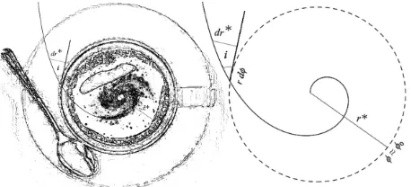
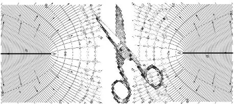
geometry along these special regions is rather uniform, the test orbiting bodies receive the same code of instruc- tions, and the unexplained stiffness in the geometry is primarily due-according to the launched hypothesis-to a second order phase transition where the space-time ac- quires, at low curvatures, the properties of a superfluid. Basically, Weizsaecker’s “coffee-cup” analogy [1] is re- placed by a “superfluid-cup” one, where phonons and ro- tons can flow, see Figure 1.
Can the geodesic motion of a radial alignment of test particles resist the winding process when the space-time is a superfluid [5,6]? How, in the first place, do quantum vortices behave if the space-time is a superfluid? In this article a research program is commenced by examining fully this second opening issue.
It should be stressed that the catalog of spiral galaxies is indeed vast: the so called grand design spirals have a well defined two-arm structure, but some others present multiple arms not necessarily symmetrical spaced, while there are others-referred to as flocculent spirals-showing sporadic spiral arm segments [5]; spiral patterns of a very
Figure 1.Left: coffee-cup analogy. Right: winding dilemma. Let and be respectively the radial distance to a cen- tral point and the local spherical radius. If a thin disk of matter rotates around such a point with an angular velocity and if then, an original aligned confi- guration
r
r
r
0,
, 0;
r
or t
of physical bodies belonging to the disk will transform, over time, into a spiral arm with a pitching angle approxi- mately given by
i
i r
cot d
r
220 k
r r r t t
d d d ; 0.
And when the local spherical radius is assumed to chan-
ge as the radial distance r , i.e. it is
concluded that for typical galaxies the spiral arm must be tightly wound, contrary to observation. A rotational velo- city
(i.e.
r
rrconstant,
1
m s 1r)
i0.25
, ,
and implies as well as an interarm
separation of [see [5]]. Presumably such alleged relationship between and r
rr10 Kpc t 10
10 yr 0.28 Kpc
r breaks down in spiral ga- laxies [6].
bizarre shape also show up in Nature: for instance, the spiral galaxy NGC4622 not only posses inner spiral arms that are trailing but also has a pair of outer arms that are leading, contrary to most expectations [7]. The oddest thing of all is that according to standard theory, if the material originally making up a spiral arm remains in the arm; then, the differential rotation of the galaxy will wind up the arm in a time short compare with the age of the galaxy. But most spiral arms (often logarithmic in nature) are far from being too tightly wound, with a pitch
angle absolute value ranging from 6 to [8-10].
How can this be?
27
This acute observation creates a fundamental challen- ge to theories on the origin of the spiral structure and it is referred to as “the winding dilemma” [11]. A description of this winding process, when there is an annular disk of material with a constant pattern speed-thus fulfilling the flat rotation curve criterion-is given in Figure 1.
At first sight, these bearings seem no different if one assumes that the orbiting objects are governed by Kepler’s laws of planetary motion or if they move with an approximately constant pattern speed; that is why, in
the 1960s, an hypothesis was advanced: where the spiral features were assumed not only to be long lasting, but also that they were the result of a quasi-stationary density wave that rotated rigidly, at a slow paced rate, through the galactic disk-meaning in particular that stars should stream in and out of the spiral arms as they orbit the gala- xy. This theory, however, has not been satisfactorily con- firmed as even the question of longevity of the spiral arms, whether they are short-live transient patters (per- haps breaking apart and reforming periodically) or not has not yet been settled [12,13]. In Binney & Tremaine comprehensive treatise on galaxy formation this peculiar situation is depicted as follows [5]:
“The common thread of several of these mechanism is that because of the swing amplifier, galactic disk respond with remarkable vigor to a wide variety of perturbations, whether these be tidal forces, gravitational instability of some local pattern of gas or stars, or fresh leading density waves. In some cases there is clear evidence that Lindblad’s original conception of the spiral arm as a density wave is correct. However, there is little or no direct evidence for the hypothesis that the spiral pattern is stationary (i.e. that it looks the same in 109 yr or so).”
Intriguingly, if the density wave theory were correct, a spatial ordering of different stages of star formation would be expected in the arms of galaxies: with very young objects on the leading edges of the arm (where star birth would be triggered by a compression wave) and the oldest ones on the trailing edge. However, research involving computer algorithms to examine twelve nearby spiral galaxies of different variety: such as the ‘whirlpool galaxy’ M51a, M63, M66, M74,and M95-an interacting, a flocculent, an arm-distorted, a grand design, and a barred spiral respectively-did not find such an ordering, leading to the conclusion that spiral density waves in their simplest form are not an important aspect of explaining spirals in large disk galaxies [14].
The purpose of this article is two fold:
Firstly: to get a deeper understanding of the physics of rotating astrophysical bodies in models where the space- time exhibits non trivial macroscopic quantum effects.
Secondly: to deduce, in some quantitative way, part of the relevant signatures (topological traces) which might help to reveal whether or not such exotic behaviour is present in our universe.
a role analogous to an electric charge. Finally, the basic results are discussed and summarised in Section 9, where future directions for research are indicated.
2. Space-Time as a Charged Superfluid
In the late 1930s, W. H. Kessom, P. Kapitza, J. F. Allen and A. D. Misener, initiated a series of low-temperature experiments that led to the discovery of superfluidity [15,16], a quantum many-body effect responsible of very striking properties in a superfluid, such as: an infinity heat conductivity, i.e. the boiling abruptly stops, a zero viscosity (superleaking with zero resistance), the fountain and mechanocaloric effects, to cite some appearing below a certain critical temperature (the - point for He II) and strictly at speeds under some critical velocity Vc.
Is the space-time at galactic scales acting as a super- fluid?
According to the prevailing view, at extragalactic sca- les the expanding universe is best think of as consisting of two parts: one luminous (obeying Newtonian mecha- nics in the limit of slowly moving bodies and large dis- tances) and the other dark, or to use perhaps a better word: invisible (which is several times more abundant than the first one, and from which the formation and sta- bility of the large scale structure of the universe pre- sumably rests upon). For this second component, the quality of being invisible (or dark) is bring at front since it is only through its gravitational interaction with other bodies that this hypothetical form of matter (so far) has been accounted for.
In our view, the whole mystery of cold dark matter, and thus, the appearance of a two-fluid like model to des- cribe the universe, where one component is behaving normally, while the other posses very odd properties, is a symptom of a bigger crisis than the one usually cured by just adding a new type of particle:
It is the failure of a proper understanding of how the quanta of mass-energy “there” rules inertia “here”. In- deed much is gained by flipping from the dark matter perspective into the realm of quantum gravitational phe- nomena, since there is now-as D. Hilbert could have put it, “a guide post on the mazy paths of hidden truths” for quantizing the gravitational field. “Quantum gravity is a very tough problem”-warned W. Pauli to B. S. De-Witt [17,18]. How are we going to unify “the strange world”
of Max Born’s probability wave amplitudes ‘s with
the peculiarities of the Einstein’s four-dimensional curved space-time continuum ?
Perhaps, as the dark mater conundrum seems to imply, we have various clues already:
There is an electrically neutral, QCD colourless, quasi- substance with local (or non-local) mass that is in a cold, stable (or long-lived) unexcited state far away of any strong field; it flows freely (without resistance) but only
at non relativistic speeds-as if there were a limiting velo- city that it cannot surpass, it has a negligible nongra- vitational interaction with ordinary baryonic matter or it- self.
What could it be? To cope with the subtleties imposed by the above scenario let us turn to mathematics since as Max Born put it [19]: “When in conflict, mathematics— as often happens—is cleverer than interpretative thought.”
3. Quantum Mathematical Model
In 1956 W. Pauli remarked [20]:
“The question of whether Kaluza’s formalism has any future in physics is thus leading to the more general un- solved main problem of accomplishing a synthesis be- tween the general theory of relativity and quantum me- chanics.”
A deep connection between Einstein’s law of gravity (with a nonzero cosmological constant) and quantum phy- sical phenomena better associated to the theory of super- conductivity was explored in [6], where the Kaluza- Klein idea of splitting the space-time metric as:
2 42 2
ds N dt A x kd k ijdx xid ,j (1)
and thus:
2 2
00 0
4
2 2
0
,
k k
i ik i ik i
N N A
g g
g
g g N A N A A
k
(2)
was adapted to offer a phenomenological, Ginzburg- Landau model of a 4-dimensional “quantum space-time”.
k
A is the gravitomagnetic vector potential, is a sca- lar field, and ij
N
is referred to as the 3-space base me-
tric. The novelty of this approach is that although all the
metric components are held real, is set to be a
complex scalar field:
1 2
exp ie ,
(3)
characterising the onset of order of a phase transition affecting the intrinsic features of the space-time itself, which-at galactic scales, it is imagined developing the properties of a highly coherent quantum system in parallelism with superfluids, lasers, and superconductors.
,
in other words, is a measure of symmetry violation. will play the role of a Goldstone boson field.
Every direct comparison between this and the (tradi- tional) ADM setting should always kept in mind the dual transformation:
; ADM
ADM
g g g g . (4)
(4).
Key points of this bold proposal are briefly described next, leaving the details to the original article, where the theory was first developed [6]. First pay attention that by
virtue of the complex nature of the scheme by H.
Weyl [21-24] to unite general relativity with electro- magnetism can be adapted to treat the gravitomagnetic field
,
,
k
A so that in theory, the primeval gauge transfor- mations set by:
exp ie ,
(5)
and
; 1, 2,
k
k k k
A A A x k 3, (6) become a symmetry of the physical gravitating system. Weyl’s original view of a 4-dimensional conformally invariant universe (described by a conformally invariant action where only purely real exponents get involved in the gauge transformation laws) was abandoned as a model for the actual state of the universe: for as much as the prediction that physical observables, such as the leng- ths and times of measuring rods and clocks, would de- pend of their prehistory, which would in turn introduce spectral blur effects which simply do not show up in reality [20,24]. Yet, gauge invariance (which has been very successful as guidance principle for formulating the electroweak and the strong nuclear interactions) can be incorporated into gravitation in another way [6] which seems more in unison with the principles of quantum mechanics.
As it is argue in pages to come, an utterly natural, Ginzburg-Landau-action principle for gravitation is:
2
1 2
, ,
2
6 3 2
2
2
1 2
2
4
12 1
4
2
det d , 8
ij
s i i
k k
ik jm ij km
e A A
e R
N
N
F F N V
j j
(7)
where the third term plainly depends on the Ricci scalar of the 3-space, base metric ij. By keeping fixed,
the -term becomes a constant multiplying the physi-
cal four-volume. Thus,
N
6
2 N2
Equation (7) is expected to be valid in stationary situations, where the temporal variations of the gravito- magnetic vector potential Ai and the base metric ij can be neglected [6]. It is exactly in this case when the parallelism between gravitation and a metallic super conductor looks more straightforward, after all, stationa- ry space-times with horizons follow mechanical rules re- sembling the laws of thermodynamics [25]. In light of this, it can be stated that the infrared quantum macro- scopic effects inherent to gravity seem best fitted by a word introduced by Kamerlingh Onnes in 1911, namely “superconductivity”.
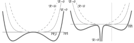
Significant aspects of this action are immediately assessed by taking a look to the condensation energy: having both a sixth and inverse-square power terms, and depicted in Figure 2. Its shape is dictated by the Eins-
tein-Hilbert action itself. Indeed, by varying and
, i
A the least action principle (7) leads respectively to the energy and momentum constraint equations of Eins- tein’s theory of gravity, as it was developed by A. Lichnerowicz, J. W. York, and Y. Choquet-Bruhat in the 40s and 80s [26,27].
The mere existence of a phase in the ubiquitous complex gravitational potential introduced in (3) and (7) has the most amazing implications [6]:
Firstly:it allows the generation of supercurrents:
2
2
,
k k
e
k
J A
N
(8)
transporting vacuum energy while deforming the gravito- magnetic (or gyrogravitational) lines of force. Be aware that closed strings are natural carriers of vacuum energy.
[image:4.595.306.540.483.559.2]Secondly:second-order phase transitions controlled by
Figure 2. Phenomenological condensation energy affecting the nature of the space-time itself. On the left, the gravito- magnetic field is switched off: in close analogy with the Meissner-Ochsenfeld effect of the theory of super conduc- tivity of metals. It is present, however, on the right side. There is a local minimum at 0 for 3R< 0 and at
s
for The negative blow up of the con- densation potential exhibited on the right is expected to be cut off by matter or hidden deep inside an absolute event horizon (in the black hole case
3 R> 0.
vanishes at the sin- gularity). The vertical line indicates the value taken by at the event horizon, usually this becomes a minimum if the space-time is restricted to lie within an isotropic coordinate chart.
e can be identified with a
vacuum energy, and must be proportional to the
only constant present in the classical Einstein’s field equations which surely, is completely determined by the microphysics of the gravitating system, expressly, Einstein’s (1917) cosmological constant. The gravito- magnetic field-stress tensor is given by ik k i, i k,
2 e
F A A
the curving of space can set in, subtlety raising the mass of the gravitomagnetic vector potential Ak, due to its inter- action with an all-pervading gravitational degree of freedom [6]: expressly, the modulus of the complex potential .
Thirdly: when a spinning point-like mass in empty space gets surrounded by supercurrents, the net effect is the generation of space-time superconducting zones, in which the associated rotation curves display non Kep- lerian features such as the ones exhibited in large spiral galaxies. Such rotations curves can be regarded as arising
from the spontaneous breaking of -symmetry
induced by the condensation of a Goldstone field coor- dinate
1 U to an azimuthal angular value; thus, defining a preferred orbital direction of reference [see [6]].
Finally: at short distances, covering only a sufficiently
small open neighbourhood of the space-time, when
(and henceforth ) has not too much relevance, the pre- dictions of Einstein’s theory of gravity are recovered. The same is truth if vanishes identically.
e
e
How does this work? Well, the string and monopole cases are provided below.
Notation and nomenclature—it is convenient to denote by s , the value taken by the modulus of the complex
field under the peculiar situation when: at
the minimum of the condensation potential. The identity:
Fij0,
2 4 1 3
6 2
s N e R
(9)
is then a direct consequence of this definition, see Figure
2. Direct inspection to (7) suggest that is physi-
cally related to a measurable mass [6].
3R
Write next
2
,
s
s (10)
and set
2 22 2
4 e N ,
(11)
also demanding that
1 2
3 3
2 R ; R
0 . (12)
is called the “London parameter” (or the penetration depth) and is referred to as the “correlation length”.
The physical significance of all these expressions will be worked out with examples later.
Equations (11) and (12) give a dimensionless Ginzburg- Landau (G-L) parameter:
(13)
equal to three halves, in line with type II super-conduc- tivity. The (G-L) parameter, however, changes its value if one allows the
e N
26-term to be multiplied by a different coefficient than 12. This arbitrariness is dis- cussed in more detail in [6]. A space-time fulfilling a principle of least action of the form given by (7) will besaid to be a charged, space-time superfluid.
Space-time defects (mathematical preliminaries): Let the initial-data hypersurface
3t,ij
be a Riemannian space of constant sectional curvature; that is to say: 3
2 ,
kl k l k l
ij i j j i
R K
(14)where K is a given constant. Then, according to the
theorem of H. Hopf and W. Killing [28,29], locally that space is isometric to one of the following models: a
3-sphere
3 , a 3-Euclidean space
, or an hy-perbolic 3-space
3
3. K
, with the same Ricci-scalar curvature 3R12 Setting K as appropriated line elements for the neighbourhood containing a given point
2
, l
3 t
p as origin are:
3
2 2 2 2 2 2 2
d d sin d sin d ,
l
s l
(15)
3
2 2 2 2 2 2
ds dr r d sin d , (16)
and
3
2 2 2 2 2 2 2
d d sinh d sin d
l
s l , (17)
in the spherical, Euclidean, and hyperbolic instances respectively. By (17), the associated Laplace-Beltrami operator
3 3R f
can be written as:
3
3 3 2
,
2 2 ,
2 2
, , ,
1
sinh sinh
1
sin sin 12 ,
sin
l R f l f
f f l f
(18)
Defining r l gives:
2
2 2 2
4 6
sinh 1 1 3
2 45 ,
l r
r l r l
r l
2 4
2 2 2
sin 1 1 3 1 90 .
l r r l r l r l 6
Since
3
2 2
, , , , 2
1 1
sin ,
sin sin
r r
f r r f f f
,
the following identity must be satisfied:
3 3
3 3
2
2 4 4 4
, , 12
1
, 3
l
r r
R f f
l
r l f r r f r l
(19)
likewise,
3 3
3
2 3
2
4
4 4
, ,
12 1
3
.
l
r r
R f f r l
l
f r r f r l
The nomenclature introduced in this passage as well as the pair set by (19) and (20), find an immediate applica- tion in the analysis of topological space-time defects, coming next.
4. String Solution
The most basic features of the line defects predicted by the quantum rule set down by (7) are determined by the set of equations:
2 2
2
,rr ,r 2 2 1 ,r ln ,r
s
r
r A rA A r rA
0, (21)
3
1 2 2 1 2
, ,
4 2
8 8 2
2 1 0,
r r
s
r r e A N H
2
(22)
where A is a scalar field; s, , and are given by (9), (10), (11), and (12) respectively; H is referred to as the gravitomagnetic field and it is given by
. H A
This can be found as follows. As in the previous
paragraph, let be a Riemannian space of constant
sectional curvature. Let 3 t
1, r l
i.e. allow the cur-
vature radius of the universe be large enough. Then, by (20), at leading order it must be true that
3 3
3 3
,
l R f R f
and similarly with other expressions having the di- vergence, the gradient, and so on-as it is intuitive from (15) and (17). Thus, it is seen that there exists a con- venient way to promote various calculations in flat space to curve space. Following this simplifying lead, make the subsequent choices. Employing cylindrical coordinates,
write H as Then, in the corresponding
orthonormal frame, the gradient of
B B Br; ; z
. and the curl of
H (or any other vector field) have respectively the
form:
1,r rˆ r , ˆ ,zˆ ,r;r ,; z
e e e 1
, , (23)
and
1
, , , ,
1
, ,
; ;
. z z r z z r
r r
r B B B B
r rB B
H
(24)
Assuming that not far away from the axis of symmetry, here symbolized by the z-axis, the “probability-like” current density:
2
1 1 1
2
,
k k k
k k
J eA
N i i
e
A
N
girdles always in the azimuthal direction, and moreover,
that its magnitude at any given point proximate
to the centre line only depends on its geodesic distance to such line, let
3 t
q
A take the form:
1 ˆ
ˆ , ; , ; ˆ
0; ; 0 .
r r r z z
A r
,
A A A A
(26)
These restrictions immediately imply:
1
, 0; 0;r rA r ,
H A (27)
and henceforth:
1 2
, , ,
0;Bz r; 0 0;Arr r A r r ; 0 .
H A (28)
Additionally, if only the radial part of the modulus
field is considered [see (3)], Combining (10) and
(11) with the Euler-Lagrange equation:
2 2 2 2 2
4 l
l l
l k k k k l
N F e A N F n , (29)
resulting from the variation A in the action principle set by (7), a differential relationship between the two unknown functions: A r
A
ˆ and2 ,
follows immediately:
2 2
2
,rr ,r 2 2 1 ,r ln ,r 0
s r
r A rA A r rA
.
(30)
By letting further, the order parameter to be a
function of only, the Lichnerowicz equation, obtained by the
r
-variation of the Ginzburg-Landau action set
by (7), becomes at leading order [using (12) and (20)]:
3
1 2 2 1 2
, ,
4 2
8 8 2
2 1 0,
r r
s
r r e A N H
2
(31)
completing the system, where the relation: km
2
2
km
F F H
entailing the gravitomagnetic field H, has been used.
4.1. Asymptotic Analysis near the String Axis
The action principle set by (7) implies the following: Firstly: the vortex-gravitomagnetic flux is quantized. Secondly: the minimal flux o is achieved by
some regular
k eA
(25)
e
II
-vortex profile. Thirdly: the order - parameter for such a vortex of minimal vorticity vanishes in a linear fashion, along cylindrical ring-like structures of nonzero finite radius. Fourhtly: near the vortex core, the asymptotic metrical aspects of the quantum, regular vortex of minimal vorticity are determined (say at the initial time t0) by
2 2
2 2
min
2
2 2 2 2 2
d d 2 d 1 3
2 d d d ,
s N c t rB r r r
N rB r r z
1
B is here the intensity of the gravitomagnetic field along the flux tube and it is assumed to be nonzero. Finally but not least-by (58), a natural way to express the fitting “charge” e is in the form e q , where
is Planck’s constant joule-seconds, mean-
ing that can be regarded as introducing an
h
34 6.626 10
h2
fac- tor into the main gravitational equations.
Proof: For the sake of argument, ignore first the A-ρ coupling in (21). Then, at sufficiently close distance from the axis of symmetry, when
1 22 2
r
and =r l1, (21) implies:
2 ; 0A r Br C er r , (32)
where and are integration constants. Inserting
(32) into (27) shows that the -constant physically gives
the intensity of the gravitomagnetic field along
the -axis, i.e.
B C
B
A z
B B Br; ; z
B
A
0; 0;B
. (33) Setting4 , NB
(34)
(22) reads, in the limit imposed by (32), as
4
2 2 2 2
,rr ,r 0; 0 .
r r r C r (35)
Equation (35) is reminiscent of the Bessel differential equation; however, it contains the non-linear 4-fac- tor, multiplying 2 and spoiling an all-encompassing similarity. To solve (35), follow these simple steps:
Firstly: verify the expression below is an exact, regular solution.
1 2
1 2 1 4 2
; 1
1 4
r r C
C
2. (36)
Secondly: spot that clearly another regular asymptotic answer is given by:
2 2 2; 0 ; 1 2
C C
r r a r r C
: (37)
whenever r0 . What about the distinctive C 1 2
value? Well, several transformations simplify the prob- lem.
Last step: as suggested by (36) and (37), pick
1 2
C (38)
and set
1 2
.
r r f r
Then, (35) reduces to
2 2 2 2 3
,r r 0,
r r f r f
r
(39)
which is symmetric under the specular transformation: By the change of variables:
.
r 1
,
r it trans-
forms into
2 3 2
, 0,
f f (40)
complying with the canonical form of the so-called Emdem-Fowler (E-F) equation:
, .
m n
y ky (41)
If m0, the E-F equation has the exact solution:
1 1 2 2 1
2 1 1
m n
y n n m k m
m (42)
as it is readily verified. Unfortunately m 3 and
2, n
thus no formal solution can be extracted from this previous knowledge, as the coefficient multiplying
2 1
n
m
diverges. To advance further, introduce the change of variable exp
t , then, (40) becomes ins- tead:2 3
,tt ,t 0,
f f f (43)
which has coefficients which do not depend explicitly on the independent t-variable. A standard trick is then to pick u t
f,t, hence f,tt uu,f, and (43) simplifies to:
2 3,f 1
u f u
, (44)which is intended to be solved for Thus, pro-
ceeding in the reverse order,
. u u f
f f r is obtained by
inverting (if possible)
d
e f u f .
r (45) The general features of the solutions, u u f
, of (44) are depicted in the phase diagram: u versus f inFigure 3. The vertical axis not only gives a measure of the magnitude of u t
f,t but also of as canbe seen by the chain of relations , .
,r,
rf
,t f, rfr
u f
r f r
Thus, the locus of points of the form where,
as a function of ,
,
r f is an extremum are mapped into
the horizontal axis
f r
, 0
of Figure 3; the points set by
f u f,
where, as a function of f, u f
2 3
u f is an
extremum falls over the dotted curve label-
ed by the latin symbol in Figure 3 Use next (44) to obtain
a
2 6 3 2 2 3 2
,ff 3 .
u f u f u f u
(46)
The superior (and by the same note, inferior) branch of the “inflexion curve”:
1 1 4 2 2
6 12
u f f f
, (47)
drew from (46) by the condition , is labeled
(jointly ) in Figure 3. The solutions can be
separated into two distinct classes, referred to as type I and type II for definiteness. A representative of each cla- ss has been found numerically and depicted in the same figure: type-I solutions do not cross the
0,
ff
u
ub
c u u f
Figure 3. Phase space: f,t versus f ( u versus f ).
type-II make that cross. Let be a type-I solution,
clearly
Iu f
I
u is bounded from below by some positive
constant, lets say uI
f . By (44), as 2k f approa-
ch infinity, u,f tends to 1. This means that uI
f takes the asymptotic form
I N
u f f f uN
as f ,
where
f uN, N is a point in
f u, I
f
. Therefore,according to (45) one has
d e ofN I
,
f u f
N N N
r u f f u (48)
as f . Meaning, by inverting the relation, that
1 2 d 1 2e ofN f uI f ;
I r fN uN r uN r r
0. (49)
The important point to make is that this is not a regular solution, since
d e ofN f uI f
N u
is obviously different from zero. Turning now to type-II solu- tions, consider the situation when one has both:
and
u 0.
f
Applying l’Hôpital’s rule to (44), it is established that in this regime:
2 2 2,f 1 ,f 3
u u u f
, (50)which gives
2 2 2
,
2 3 2 2 2
1 1 3
1 1 3
f
u u f
uf u f
.
0
(51)
Thus 3f u2 2f u3 2 and henceforth
2 4
6 1 1 12 3 .
II
u f f f f
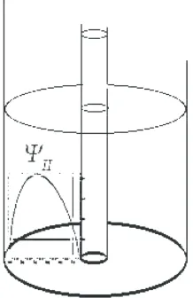
[image:8.595.369.478.87.255.2]Inserting such an expression in (45), the following asymptotic formulae for the -field are obtained, from which some characteristics observed on Figure 4 are de- duced:
Figure 4. An inner, quantum, regular vortex of minimal flux, upheld by two-coaxial cylinders of different radii, and Stick to the inner cylinder, the core of the vortex, extending even further by a distance controlled by the cohe- rent length
rmax
rmin.
,
is shielded by an annular cylindrical domain where the space-time becomes superconducting: a quantum effect accurately described by the gravitational potential:
II
r . The space-time settles down to its normal state in the neighbourhood of the outermost cylinder, where II
r vanishes as an 1
r rmax
1 2 power.
2
max
max
2 3 1
if 0; 1 2 ,
II
r r r r r
r r C
;
(52)
2
min
min
2 3 1
if 0; 1 2.
II
r r r r r
r r C
;
(53)
Let
1 22 2
min
0r r
and insert the (53) result into (21), it gives a linear non homogeneous equation whose general solution for is the sum of a particular solution, say
0 r
,V r to the solu-
tion of the homogeneous problem given by (32) again, choosing a particular solution satisfying the initial condi- tions: V V ,r0 at r r c (where c is the value of
the coordinate radius at some point of the permitted inter- val), it is seen then that the non particular solution can
only bring quadratic -corrections to the previous
answer. The
r
2c
r r
C er term in (32) still dominates the limi- ting behaviour at small radii. Thus, if
1ˆ , 2 ; 0
A r Ar Br C er r , (54)
it is consistent to set
ˆ r Br 2; r 0 ,
A (55)
C e
o
o; r 0
. (56)
Yet, the Friedmann-Lemaître-Robertson-W sc
alker-like ale factor introduced in the Kaluza-Klein-like metric (1), that is to say, the e2ie
piece, must be a
single-valued function. N y restriction on the
polar angle ,
ot having an
it must be true, if 0, that
2;
C n n, (57)
implying in turn a quantum law over the allowed values for the gravitomagnetic flux, namely
d d
H S
A sd ; ,
flux
n e n
s
(58)
in the understanding that is a planar, smooth, closed o
curve of winding number ne, surrounding the axis of
symmetry; each point of , it is assumed also, falls deep inside a large enough zone where the space-time be-
comes superconducting, and thus where A vani-
shes identically. This type of flux quantization has exact- ly the same form than in metallic superconductors, where the carriers of electric current consist of pairs of electrons. A pair of charged quantum fields , actually a field coupled to itself, appears instead in the line element (1) from which the action principle (7) is based on. Here, the fitting charge, however, is in essence pure vacuum ener- gy.
The law of gravitation (7) outlines the Bose-Einstein co
the cause of those pr
much rarer within the de
n is the intensity of what we call Gra- vi
4.2. Far Away Asymptotics
beys the asymptotic for-
ndensation of wave-particle pairs and it bring us closer to some of the most fundamental queries posed by New- ton about the origin gravity [30,31]:
“I have not been able to discover
operties of gravity from phenomena, and I frame no hypotheses; for whatever is not deduced from the pheno- mena is to be called a hypothesis, and hypotheses, whe- ther metaphysical or physical, whether of occult qualities or mechanical, have no place in experimental philoso- phy.”—Principia 2nd edition.
“Is not this Æthereal Medium
nse Bodies of the Sun, Stars, Planets and Comets, than in empty celestial Spaces between them? And in passing from them to great distances, doth it not grow denser and denser perpetually, and thereby cause gravity of those great Bodies toward one another, and of their parts towards the Bodies; every Body endeavouring to go from the denser parts of the Medium towards the rarer?” — Opticks Query 21.
In what proportio
ty affected by an increase in mass of the gyromagnetic field which, by a Higgs-like mechanism, gets transfor- med as we move further and further away from macro- scopic dense Bodies like the Sun, Stars, Planets and Co- mets? Is the local spherical radius on the verge of
becoming rather uniform so that orbiting test bodies like Stars at different radii move through paths of almost equal length? And how this rigidity (or uniformity) of the space distorts a beam of light when it departs from a point where gravity is normal, then—as it travels—the gyro- gravitational field becomes massive, to finally end at another point where the spacetime is not superconducting? Is this a step forward towards a consisitent solution to the stabilization problem of spiral galaxies?
A regular, infinite, string line, o
mulae provided below if the conditions s and
r are met:
2
cos ,
4
s o
r r
(59)
1
,2
A r K r
e
(60)
where K r1
is the Macdonald function, decaying with distance at leading order as
2 expr r .
To look for the asymptotic distance decay of the gravi- ta
tional -potential, turn back to the basic system of cylindrically symmetric equations:
2
2
2
,rr ,r 2 1 ,r ln ,r 0
s
r A rA r A r rA
(61)
41 2
4
, ,
3
2 2 2 2
8 2 1
1
8 0
2
r r
s
r r
e A N H
,
(62)
As the gravitomagnetic vector potential becomes pure gauge, as the space-time becomes superconducting, the
-field becomes, to a high degree of accuracy, given
an asymptotic expansion of the form: by
0 1 2
0 1 2
, ,
s
(63)
the system (61) and (62), in the limit
r , ,
simplifies to:
2 2
,rr ,r 2 1 0
r
r A rA A
,
(64)
and
2 2
,rr ,r 2 0 0
r
r r
.
Put attention that the A nd order
th
coupling implied by
is relevant only at seco and be alert
sim e coefficient a
(61) on the dis-
ilarity in sign between ccompanying
our correlation length and the one encountered in
standard superconductivity: our sign, one may say, is anomalous. Nevertheless, this does not seem to represent a severe problem; on the contrary, it is necessary to dis- play some of the features observed for the shape of the galactic rotation curves, as it is argued in [6]. (64) is just the modified Bessel equation:
22 2 2 2
d d d d 0.
z w z z w z z w
(66)
and it has as one of its solutions: the Macdonald function
,K z decaying exponentially to zero according to
the asymptotic representation [32]:
2
4 1
e 1
2 1!8
z
K z
z z
2 2 2
2 2
2 2 2 2 2
3 3
4 1 4 3
2! 8
4 1 4 3 4 5
1 . 3! 8
z
z z
(67)
One discards the other independent solution, the hy- perbolic Bessel function of the first kind
,I z sin-
ce it grows exponentially with z, giving an apposite effect not in line with (63), unless s be unbounded. In the next section a rough estimate of the vortex-vortex interaction energy is obtained with the help of some iden- tities satisfied by the Macdonald function, which for con- venience’s sake are listed here: namely, its divergent be- haviour at the origin:
2 If 0, 0 ,
2 z z
ln z 2 If 0,
K z
1
1
lim nk ln ,
n k n
(68)where is the Euler-Mascaroni consta ly given by
nt, approximate-
0.5772156649015328606065121,
and the differential identities:
1
1
d
,
dz z K z z K z
(69)
1
1
d
.
dz z K z z K z
In the same train of thought, (65) is just the Bessel o.d.e:
(70)
22 2 2 2
d d d d 0,
z w z z w z z w
w
(71)
hich has as solutions the cylindrical harmonics J z
and Y z
. An asymptotic representation of them for large real arguments is given respectively by
2cos
2 4
J r
r
and
r
(72)
2sin
2 4
r Y r
r
(73)
if 2
1 4 .
r
tory an
Their distance decay is thus oscilla-
d modulated, in part by the two-dimensional na- ture of the problem, by an inverse square ro
the separation distance from the source. No ort radii:
ot power of netheless at sh
2ln 2 if 0
o
Y z z z
(74)
holds.
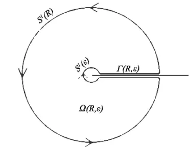
Now, consider the Green’s identity:
,
.
o o
R
f K r K r f
K r
, o
o R
f
f K r
n
n
(75)
over the contour
depicted in Figure 5, letting f
be
a regular function on
R, —we already (68), thatknow, by
o K r g
is i gular there. Ad
subtractin
ndeed re ding and
2 o
fK r
to the integrand on left hand
[image:10.595.322.508.487.631.2] [image:10.595.78.288.506.582.2]side of (75), and usi g (66), we get: n
Figure 5. Contour path
R,
ac delta diof zero winding number, used to define the Dir stribution 2
rurve
in a cylindrically symmetric space. The planar c
R,
is composed of two concentric circles S1
and
S R of arbitrarily small and large ii respectively, as well as of two antiparallel segments along the nonnegativ semi-1
rad
,
2
,
.
o o
R
o R
f K r K r f
K r f
)
But the right-hand sid
(76
e of (75) is the sum of two con- tour integrals: one along the circle of very large radius
where the asymptotic representation o the other along the circle of small radius
1
S R lies, and
f (67) app-
1
S
ing the where (
lim
68) holds asymptotically. Therefore, tak it
R,
, 0
gives
2
,0 , 0
lim o 2 lim ,
R
K r f f
(77)
on the assumption that not only
, R
2 2
C 0
f
is bounded from above
f M
outside a disk of sufficiently large radius, but also that2
B
0
lim ln 0.
r
f
r r
r
(78)
chwartz’ butions,
Following Laurent S s theory of distri
a linear map
2
: ,
o
K r
from a proper space of test functions to the reals can th
en be defined with the help of (77), symbolically written as:
2
2
2 ,
o
K r r
(79)
ta
where 2
r : is Dirac’s del distribution with support at the polar origin. Likewise (73) and (74) leads to
2
4 2 o
Y r r
ware, however
of boundary terms in the far field regime, in more diverse applications, stronger assumptions tha
required for making sense of (79) must apply a
t,
. (80)
Be a , that as the natural space of test
functions should be in tune with the vanishing hypo- thesis
n the ones (if needed, change of measure under which the given integrals are
carried ou say by adding proper weighting factors be-
comes a natural way to follow). Proceeding on such grounds it must be true, by (66) and (67), that
1
; ,2 s
A r K r
e
(81)
which by (27), (69), and (79), immediately gives
1 ,
, , ,
2
2 2
.
2 2
z r r o r r
o o
r e e
K r K r
e e
ression is expected. Combining (72) and (73), we get
1 1
1
B rA r rK r rK
(82)
The minus sign appearing at the end of this exp
1 2
cos ,
4 o
s o
r r
(83)
where o (determining the first order of the perturba-
tion amplitude) and (the angular phase) are integra- tion constants. An immediate application of (59) and (60) is the estimation of the vortex-vortex and vortex vortex interaction energies.
by:
(84) -anti-
5. Spin Interaction
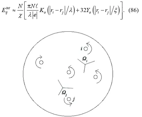
Imagine a large pattern of quantum, space-time vortices: each vortex labelled by a unique number ,i whose axes are all aligned, as depicted in Figure 6. Let the Lagran- gian of the system be given
0 1 2
.
int intint system free
0
denoting the free Lagrangian: free, approximately
given by a sum over disjoint regions of space
ri (hereafter referred to as terminals or ends) of compact support centred at each space-time quantum vortex: each vortex treated at leading order as if it were in com isolation, plus a remainder; that is to say:(85
an interaction energy given by:
plete
free remainder
i
r i
)
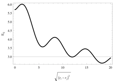
where is given by (7). To a good degree of accuracy, two stationary, axis-aligned, quantum space-time vortices with the same sense of spin, interact with
32
.int
ij o i j o i j
E K r r Y r r
e
N N
(86)
[image:11.595.313.544.477.667.2]