ISSN: 1992-8645 www.jatit.org E-ISSN: 1817-3195
AN IMPROVED PARTICLE SWARM OPTIMIZATION
ALGORITHM FOR PROTEIN STRUCTURE PREDICTION
BASED ON AB MODEL
YIWEN ZHONG, JUAN LIN, XIAOYU LIN, HUI YANG
College of Computer and Information Science, Fujian Agriculture and Forestry University, Fuzhou, 350002
E-mail: [email protected] , [email protected] , [email protected] , [email protected]
ABSTRACT
An improved particle swarm optimization algorithm, which combines the idea of simulated annealing algorithm and opposition-based learning strategy, is presented for NP-hard protein structure prediction based on AB model. Flying grain is used to control the neighborhood structure of particle, so particle can search the global optimum in solution space more finely. An opposition-based learning is used to keep the diversity of swarm and improve the algorithm’s ability to escape from local optima. Furthermore, the Metropolis criterion of simulated annealing algorithm is used to balance the exploitation and exploration ability. Simulation results show that those strategies can improve the performance of the proposed algorithm effectively.
Keywords: Particle Swarm Optimization, AB Model, Protein Structure Prediction, Simulated Annealing
Algorithm, Opposition-Based Learning, Flying Grain
1. INTRODUCTION
Protein structure prediction (PSP) problem is regarded as one of the oldest, most important, yet a highly challenging problem both for the biology and for the computational communities[1]. Solution of this problem would have an enormous impact on medicine and the pharmaceutical industry, since successful tertiary structure prediction, given only the amino acid sequence information, would allow the computational screening of potential drug targets. The main difficult of this problem is the computing complexity for finding the configuration with minimum energy. PSP methods must explore the space of possible protein structures which is astronomically large. Several models, such as hydrophobic/polar (HP) model[2] and off-lattice toy (AB) model[3], were proposed to simplify the structure of proteins. Despite the simplicity of HP model and AB model, both of them are NP-hard problem. Several heuristics algorithm have been successfully applied to AB model, such as
simulated annealing (SA) algorithm[4], hybrid
evolutionary algorithm[5], genetic annealing
algorithm[6], quantum clonal selection algorithm[7], particle swarm optimization (PSO) algorithm[8-11] and differential evolution (DE) algorithm[12] etc.
PSO algorithm is a stochastic population based optimization algorithm, first published by Kennedy
to accept new velocity and position, and OBL is used to enhance the chance to escape from local optima. We analyze the performance of our algorithm on 2D PSP based on AB model.
The remainder of this paper is organized as follows: Section 2 provides a short description of PSP problem based on 2D AB model and PSO algorithm. Section 3 presents our proposed PSO algorithm with Metropolis criterion and OBL strategy. Section 4 gives the experimental approach and results of experiments carried on a Fibonacci sequence and four real protein sequences. Finally, section 5 summaries the study.
2. PRELIMINARIES
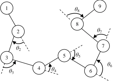
2.1 Protein Structure Prediction Problem Although a protein is formed by a combination of 20 possible standard amino acids, AB model incorporates only two “amino acids”, to be denoted by A and B, in place of the 20 that occur naturally. In 2D AB model, A represents hydrophobic amino acids and B represents hydrophilic amino acids. They are linked together by rigid unit-length (distance = 1) bonds to form linear unoriented polymers that reside in two dimensions. For any protein structure composed by N-monomers represented with the AB model, N-2 bend angles will be needed. These angles are defined in the range −π ≤θ ≤π
[image:2.612.95.287.486.624.2]i . Figure 1 is the representation of a hypothetical protein composed by nine amino acids, each one bonded to the next in the chain.
Figure 1: Generic Representation Of A Hypothetic 9-mers Protein Structure With Its Bended Angles
The energy function for a protein structure with N
monomers (N-mers) is given by equation (1):
( )
∑ ∑
(
)
∑
− = =+ − = + = 2 1 2 2 1 21 , ,
N i N i j j i ij N i
i V d
V θ ξ ξ
φ (1)
This energy function postulates that two kinds of interactions compose the intermolecular potential energy for each molecule: Backbones bend potentials (V1) and non-bonded interactions (V2). The former is independent of the A, B sequence, while the latter vary with that sequence and will receive a contribution from each pair of residues not directly attached by a backbone bond.
The backbone potential (V1) has a simple trigonometric form as follows:
( )
14 (1 cos )1 i i
V θ = ⋅ − θ (2)
The residue pair interactions (V2) which only operate between unlinked residues possess a species-dependent Lennard-Jones form as follows:
(
)
(
12(
)
6)
2dij, i, j =4⋅ dij− −C i, j ⋅dij−
V ξ ξ ξ ξ (3)
(
i j)
(
i j i j)
Cξ,ξ =18⋅1+ξ +ξ +5⋅ξ ⋅ξ (4)
where dij is the distance between residues i and j,
and the discrete variables
ξ
i denote residue speciesas follows: 2 1 2 1 1 1 2 1 1 1 sin cos 1 + + =
∑ ∑
∑ ∑
− + = =+ − + = =+ j i k k i l l j i k k i l l ijd θ θ (5)
( )
A =+1, i( )
B =−1i ξ
ξ (6)
Therefore the coefficient
C
( )
ξ
i,
ξ
j is +1 for anAA pair, +1/2 for a BB pair, and -1/2 for an AB pair. Consequently the first of these pairs may be regarded as strongly attracting, the second as weakly attracting, and the third as weakly repelling. This diversity mimics in a simple way that of real amino-acid residues, which vary in size, polarity, and degree of hydrophobicity.
2.2 Particle Swarm Optimization Algorithm There are two variants of the PSO algorithm. One has a global neighbourhood, and the other has a local neighbourhood. In the global variant, each particle moves towards its best previous position and towards the best particle in the whole swarm. In the local variant, each particle moves towards its best previous position and towards the best particle in its specified neighbourhood. Suppose that the search space is N-dimensional, then the ith particle of the swarm can be represented by an N -1 2 3 4 5 6 7 8 9 θ2
θ3 θ4
θ5
θ6
θ7
ISSN: 1992-8645 www.jatit.org E-ISSN: 1817-3195
dimensional vector, Xi = (xi1, xi2, ..., xiN). The
velocity of this particle, which represents the position change of this particle, can be represented by another N-dimensional vector Vi = (vi1, vi2, ...,
viN). The best previously visited position of the ith
particle is denoted as Pi = (pi1, pi2, …, piN). For the
global variant, the best previously visited position of the swarm is G = (g1, g2, ..., gN), and let the
superscripts denote the iteration number, then each particle is manipulated according to the following two equations:
) ( )
( 22
1 1
1 t
ij t j t
ij t ij t
ij t
ij wv cr p x cr g x
v+ = + − + − (7)
1
1 +
+ = + t
ij t ij t
ij x v
x (8)
where j =1, 2, ..., N; i =1, 2, ..., M, and M is the size of the swarm; w is called inertia weight, which is used to control the impact of the previous history of velocities on the current velocity, thus to influence the trade-off between global and local exploration abilities of the particle; c1, c2 are two positive constants, called cognitive and social parameter respectively; r1, r2 are random numbers, uniformly distributed in [0, 1]; and t =1, 2, ..., determines the iteration number. Equation (7) is used to calculate the particle’s new velocity according to its previous velocity and the distances of its current position from its own best previously visited position and the global best experience. Then the particle flies toward a new position according to equation (8). Parameter w, c1 and c2 control particle’s learning from its previous velocity, its history best position and the best position of its neighbors respectively.
3. IMPROVED PSO ALGORITHM
3.1 Flying Grain and Metropolis Criterion We define flying grain (FG) as the number of dimensions which particle updates using equation (7) and (8). In a classical PSO algorithm, FG is equal to the dimension of problem. In PSOIIS algorithm, the FG is equal to 1. After a particle has updated its velocity and position, classical PSO algorithm will accept the new velocity and position blindly, it means that the new values will be accepted always, regardless of whether they are better or worse than their original values. In PSOIIS algorithm, greedy strategy is used to decide whether to accept the new values or not. It means only those better new values will be accepted. Greedy strategy may decrease the explorability, opposite velocity is
introduced in PSOIIS to keep the diversity of swarm. Aims to get better balance between explorability and exploitability, we try to find a suitable FG for PSP problem based on AB model. And we use the Metropolis criterion of SA algorithm to decide whether to accept the new velocity and position or not. It means that particle will accept better solutions unconditionally, and it will accept those worse solutions with a probability. Suppose the energy difference between new solution and old solution is ∆E and the current temperature is t,the accepting probability is equal toexp(-∆E/t).
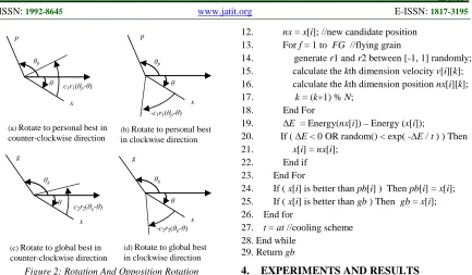
3.2 Opposition Rotation Based Learning
Even though the Metropolis criteria, which allows particle to accept worse solutions, can enhance the explorability of PSO algorithm, flying to particle’s best position and the global best position may move all particle to local optima easily and decrease the diversity of swarm quickly. Aims to overcome this shortage and consider that for PSP problem, each data x represents an angle θ in the range [-π, π], we propose a novel OBL strategy, named as opposition-rotation-based learning (ORBL). Suppose the current position is x
and personal best position is p, particle will use velocity equation to calculate angular velocity
c1r1(θp-θ); and then it will rotate to p in
counter-clockwise direction as showed in figure 2 (a). In fact, x can rotate to p in two different directions, clockwise or counter-clockwise. Inspired by this, we define an opposite rotation as rotation in clockwise direction as showed in figure 2 (b). Similarly, suppose the global best position is g, beside the angular velocity c2r2(θg-θ) in
counter-clockwise direction, we can define another opposite rotation which rotates to g in clockwise direction as showed in figure 2 (c) and (d).
The combination of ± c1r1(θp-θ) and ± c2r2(θg-θ)
Figure 2: Rotation And Opposition Rotation
3.3 Pseudo Code of Improved PSO Algorithm Algorithm 1 is the pseudo code of our improved PSO algorithm. Where x, v, and pb are all 2-dimensional arrays. The x represents positions of all particles, x[i] represents the position of ith particle, and x[i][j] represents the jth dimensional position of
ith particle. Similarly, the v represents velocities of all particles, v[i] represents the velocity of ith particle, and v[i][j] represents the jth dimensional velocity of ith particle. The pb represents best previously visited positions of swarm, pb[i] represents the best previously visited position of ith particle, and pb[i][j] represents the jth dimensional value of best previously visited position of ith particle. Variable gb is a 1-dimensional array, which represents the best previously visited position of swarm. Function Energy is used to calculate the energy of a structure specified by the position of particle. For cooling scheme of Metropolis criteria, we use the most often used exponential annealing.
Algorithm 1 Improved PSO algorithm 1. Initialize parameters w, c1, c2, fg and t0; 2. For each particle i = 1 to M
3. Generate position x[i] and velocity v[i] randomly; 4. pb[i] = x[i]; //personal best position
5. End for
6. gb = findBest( x ); //global best position 7. t = t0; //initial temperature
8. While ( End condition is not met ) 9. For each particle i = 1 to M 10. For each dimension j =1 to N 11. k = j;
12. nx = x[i]; //new candidate position 13. For f = 1 to FG //flying grain
14. generate r1 and r2 between [-1, 1] randomly; 15. calculate the kth dimension velocity v[i][k]; 16. calculate the kth dimension position nx[i][k]; 17. k = (k+1) % N;
18. End For
19. ∆E = Energy(nx[i]) – Energy (x[i]);
20. If ( ∆E < 0 OR random() < exp( -∆E / t ) ) Then 21. x[i] = nx[i];
22. End if 23. End For
24. If ( x[i] is better than pb[i] ) Then pb[i] = x[i]; 25. If ( x[i] is better than gb ) Then gb = x[i]; 26. End for
27. t = at //cooling scheme 28. End while
29. Return gb
4. EXPERIMENTS AND RESULTS
4.1 Analysis on Fibonacci Sequence
We analyze the proposed PSO algorithm using a benchmark Fibonacci sequence with 13 residues as showed in table 1. In this table, there are also results obtained by other authors using different methods. Emin is the minimum energy obtained by the conformational space annealing algorithm[16] and annealing contour Monte Carlo algorithm[17]. ELAGAA is obtained by a genetic-annealing
algorithm with local adjustment mechanism[6]. ESeq
and EDE-RI is obtained by sequential and parallel
DE with ring-island (RI) topology[12]. In order to find the suitable FG and cooling coefficient a, we fix other parameters as follows: w=0.7, c1=c2=2.0,
t0=1 and M=10. The maximum iteration times is 3000, so the total function evaluation times is 3000*10*N, which is same as in literature [8] and far less than in literature [12]. In the simulation, we change a from 0.990 to 1.000 at increments of 0.001 and change FG from 1 to 4 at increments of 1. For each combination of a and FG, we run PSO algorithm 30 times. Table 2 and table 3 are the average energy and best energy of the simulation results. In table 2 and table 3, each row means different cooling coefficient and each column means different flying grain. Those results show that: (1) Comparing different FG, our algorithm has best performance when FG is equal to 2. As showed in second column of table 2 and table 3, among the 10 different a, our algorithm has best performance in 7 cases in terms of average solution and best solution respectively, and it found the best known solution in 4 cases; (2) Comparing different a, our algorithm has best performance in terms of average -c1r1(θp-θ)
θ θp p
x
c1r1(θp-θ) θ θp p
x
(a) Rotate to personal best in counter-clockwise direction
(b) Rotate to personal best in clockwise direction
-c2r2(θg-θ) θ
θg g
x c2r2(θg-θ)
θ θg g
x
(c) Rotate to global best in counter-clockwise direction
ISSN: 1992-8645 www.jatit.org E-ISSN: 1817-3195
solution when a is equal to 0.997, and has best performance in terms of best solution when a is equal to 0.996. Among 4 different FG, our algorithm found the best known solution in 3 cases when a is equal to 0.996.
Table 1: Benchmark Fibonacci Sequence Of Length 13
Sequence Emin ELAGAA ESeq EDE-RI
[image:5.612.88.301.221.384.2]ABBABBABABBAB -3.2941 -3.2940 3.1990 -3.2924
Table 2: Average Solution Under Different Cooling Coefficient And Different Flying Grain
a FG = 1 FG = 2 FG = 3 FG = 4
0.990 -2.5813 -3.0588 -3.0506 -2.9350
0.991 -2.5852 -2.9318 -3.0363 -2.9589
0.992 -2.7322 -3.0619 -3.0554 -2.9984
0.993 -2.8013 -3.0953 -3.1359 -3.0494
0.994 -2.8069 -3.1654 -3.1293 -3.0623
0.995 -2.8785 -3.1955 -3.1184 -3.0711
0.996 -3.0268 -3.1967 -3.1892 -3.1416
0.997 -3.1051 -3.2048 -3.2041 -3.1621
0.998 -3.1535 -3.1995 -3.1969 -3.1545
[image:5.612.308.528.258.331.2]0.999 -3.0498 -3.1318 -3.1323 -3.0930
Table 3: Best Solution Under Different Cooling Coefficient And Different Flying Grain
a FG = 1 FG = 2 FG = 3 FG = 4
0.990 -3.1774 -3.1983 -3.2575 -3.1987
0.991 -3.1666 -3.2941 -3.1990 -3.2234
0.992 -3.1810 -3.2938 -3.2235 -3.1989
0.993 -3.1881 -3.2758 -3.2938 -3.1990
0.994 -3.2877 -3.2941 -3.1990 -3.1990
0.995 -3.2941 -3.2941 -3.2941 -3.1990
0.996 -3.2940 -3.2941 -3.2941 -3.2941
0.997 -3.2939 -3.2938 -3.2939 -3.2935
0.998 -3.2880 -3.2921 -3.2911 -3.1968
0.999 -3.2091 -3.2441 -3.2352 -3.2430
In order to analyze the effect of Metropolis criterion and ORBL, we compare the performance of PSO algorithm with or without those strategies. According to the results of table 2 and table 3, we set FG=2 and a=0.996. Table 4 is the simulation results of those PSO algorithms. In table 4, PSO is the basic PSO algorithm where FG is equal to N. PSOSA is PSO algorithm with Metropolis criterion of SA only, PSOORBL is PSO algorithm with ORBL strategy only, and PSOSA+ORBL is PSO algorithm with Metropolis criterion and ORBL strategies both. In those tables, ALIG is average last improving generation, which means algorithm will never find better solution after that. Those results show that: (1) although the bigger ALIG means PSO algorithm is
not easily trapped into local optima, both average solution and best solution are not good enough. The blind accept strategy and the interference between different dimensions may deteriorate the intensification ability of PSO algorithm; (2) When Metropolis criterion or ORBL strategy is used independently, the performance is not good enough also. The small ALIG means PSOSA and PSOORBL algorithm are easily trapped into local optimum. When both Metropolis criterion and ORBL strategy are used, PSOSA+ORBL algorithm has best performance.
Table 4: Performance Comparison Of PSO With Different Strategies
Algorithm Average Best Worst ALIG
PSO -2.0030 -2.7519 -1.4047 2789
PSOSA -2.0053 -2.9023 -1.3439 1333 PSOORBL -2.3052 -3.1633 1.7157 1854 PSOSA+ORBL -3.1967 -3.2941 -2.4928 2935
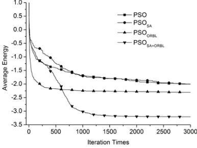
Figure 3 is the iteration process of average energy of algorithm PSO, PSOSA, PSOORBL and
PSOSA+ORBL. Figure 3 shows that: (1) although
[image:5.612.89.299.404.563.2]basic PSO has persistent optimizing ability, but the convergence speed is slow; (2) PSOORBL has good convergence speed, but it will lose optimizing ability quickly. PSOSA+ORBL has good persistent optimizing ability; (3) although PSOSA+ORBL is far better than PSOSA and PSOORBL, its optimizing speed becomes very slow in the late stage.
Figure 3: Iteration Process Of Average Energy With Different Strategies
[image:5.612.322.515.462.607.2]K-D method is used to distinguish hydrophobic and hydrophilic residues of 20 amino acids in real proteins. Briefly speaking, amino acids I, V, L, P, C, M, A, G are hydrophobic and D, E, F, H, K, N, Q, R, S, T, W, Y are polar. Table 5 is the data about those four real protein sequences. In this table, there are also results obtained by other authors using different methods. ELAGAA is obtained by a genetic-annealing algorithm with local adjustment mechanism[6]. ESPPSO is obtained by stochastic perturbation PSO combining with hill climbing algorithm[8].
Table 6 is the simulation results of PSOSA+ORBL algorithm on 1BXP, 1BXL, 1EDP and 1EDN respectively. Table 5 and table 6 show that
PSOSA+ORBL algorithm has better performance than
ELAGAA and ESPPSO algorithm on all four sequences.
It is worth to mention that our algorithm does not use hill climbing algorithm to improve the found solution, so the function evaluation times of our algorithm is less than SPPSO algorithm. The big ALIG means PSOSA+ORBL has persistent optimizing ability.
Table 5: The Four Real Protein Sequence Used In Our Experiment
PDB
ID N Sequence ELAGAA ESPPSO
1BXP 13 MRYYESSLKSYPD -2.2448 -2.4902
1BXL 16 GQVGRQLAIIGDDINR -8.7469 -8.5731
1EDP 17 CSCSSLMDKECVYFCHL -5.6072 -6.7081
[image:6.612.86.302.390.560.2]1EDN 21 CSCSSLMDKECVYFCHLDIIW -7.0961 -8.6495
Table 6: Results Obtained By PSOSA+ORBL Algorithm
PDB ID Average Best Worst ALIG
1BXP -2.2896 -2.4902 -2.1119 2972
1BXL -8.5161 -8.8126 -7.7829 2949
1EDP -6.7877 -6.9504 -6.4063 2972
1EDN -8.1118 -8.6716 -7.7062 2981
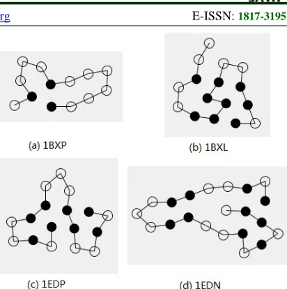
In order to evaluate visually the quality of the minimum energy configurations found by this paper, the best results were used to draw the planar form of the sequence. Figure 4 (a), (b), (c) and (d) show the minimum energy configurations found for 1BXP, 1BXL, 1EDP and 1EDN respectively. In figure 4, filled circles represent ‘A’ monomers and the unfilled circles represent ‘B’ monomers. It is easy to see that the hydrophobic (A) monomers form one hydrophobic core in the 2D AB model for 1BXP, 1BXL and 1EDP, and form two cores for 1EDN. This can be explained by the fact that hydrophobic monomers are always flanked by the hydrophilic monomers along the sequence.
Figure 4: Minimum Energy Configurations Found By The Proposed Algorithms
5. CONCLUSION AND FUTURE WORK
This paper introduces a improved PSO algorithm for 2D protein structure prediction based on AB model. Aims to deal with the interference phenomena between different dimensions, we use flying grain to control the neighborhood structure of particle, so particle can search the solution space more finely. In AB model, the range of each dimension is in [-π, π], which can be processed as a finite and unbounded circle. Inspired by this
feature, we introduce the ORBL strategy to
enhance the chance to escape from local optima. Metropolis criterion is combined into our algorithm. Those strategies can improve the balance between intensification and diversification significantly. The experiment simulations, which were carried on four real protein sequences, indicate that the proposed algorithm is promising.
Due to the high complexity of energy function of AB model, we ran the proposed algorithms on short proteins only; further study can be done on the implementation of parallel PSOSA+ORBL algorithms and its application on 2D and more complex 3D AB model for long protein sequences.
REFRENCES:
ISSN: 1992-8645 www.jatit.org E-ISSN: 1817-3195
[2] K. Dill, “A Theory for The Folding And Stability of Globular Proteins”, Biochemistry, Vol.24, No.6, 1985, pp.1501-1509.
[3] F.H. Stillinger, T. Head-Gordon, C.L. Hirschfield, “Toy Model for Protein Folding”,
Physical Review, Vol.48, No.2, 1993, pp.1469-1473.
[4] Z.R. Xu, X.M. Wang, “On Protein Folding Based on Improved Simulated Annealing Algorithm”, Computer Applications and Software, Vol.26, No.12, 2009, pp.24-26.
[5] Y.W. Zhou, P.T. Han, “Analysis of Protein Folding Using a Novel Hybrid Evolutionary Algorithm”, China Journal of Bioinformatics, Vol.8, No.1, 2010, pp.73-74, 81.
[6] X.L. Zhang, X.L. Lin, “Protein Folding Prediction Using an Improved Genetic-Annealing Algorithm”, Lecture Notes in Computer Science, Vol.4304, 2006, pp.1196-1200.
[7] F.P. Tian, J. Wu and H.B. Zhu, “A Novel Quantum Clonal Selection Algorithm for AB Off-Lattice Model Protein Folding Structure Prediction”, Journal of Wuhan University Natural Science Edition, Vol. 58, No.2, 2012, pp.144-148.
[8] H.B. Zhou, Q. LV and W. Wen, “Stochastic Perturbation PSO Algorithm for Toy Model-Based Protein Folding Problem”, Computer Engineering and Applications, Vol.47, No.18, 2011, pp.234-236,248.
[9] H. Guo, R. Lan, X. Chen and Y.X. Wang, “Tabu Search-Particle Swarm Algorithm for Protein Folding Prediction”, Computer Engineering and Applications, Vol.47, No.24, 2011, pp.46-50.
[10] C.Y. Li, Y.R. Ding and W.B. Xu, “Research of Protein Structure Prediction Based on Multiple-Layer Quantum-Behaved Particle Swarm Optimization and Toy Model”,
Computers and applied Chemistry, Vol.11, No.28, 2010, pp.1574-1578.
[11] X.L. Zhang, T.T. Li and J. Lu, “Study of Multi-PSO Algorithm for Protein Folding Prediction Problem of Toy Model”, Computer Science, Vol.35, No.10, 2008, pp.230-235.
[12] D.H. Kalegari and H.S. Lopes, “A Differential Evolution Approach for Protein Structure Optimization Using a 2D Off-Lattice Model”,
International Journal of Bio-Inspired Computation, Vol.2, No.3/4, 2010, pp.242-250. [13] J. Kennedy and R. Eberhart, “Particle Swarm
Optimization”, IEEE International Conference
on Neural Networks, Perth, Australia, 1995, pp.1942-1948.
[14] R. Eberhart and J. Kennedy, “A New Optimizer Using Particle Swarm Theory”, In: Proc of the Sixth International Symposium on Micro Machine and Human Science, Nagoya, Japan, 1995, pp.39-43.
[15] Y.W. Zhong, X. Liu, L.J. Wang, C.Y. Wang, “Particle Swarm Optimization Algorithm with Iterative Improvement Strategy for Multi-Dimensional Function Optimization Problems”,
International Journal of Innovative Computing and Applications, Vol.4, Nos.3/4, 2012, pp.223-232.
[16] S.Y. Kim, S.B. Lee, J.Y. Lee, “Structure Optimization by Conformational Space Annealing in an Off-Lattice Protein Model”,
Physical Review, Vol.72, No.1, 2005, pp. 011916.