Robust Digital Watermarking for Compressed 3D Models based on Polygonal Representation

Robust Digital Watermarking for Compressed 3D Models

based on Polygonal Representation

Samir Abou El-Seoud

Faculty of Informatics and Computer Scieence, British

University in Egypt (BUE)

Nadine Abu Rumman

Prince Sumaya University for Technology (PSUT), Jordan

Islam A.T.F. Taj-Eddin

Faculty of Informatics and Computer Scieence, British

University in Egypt (BUE)

Khalaf F. Khatatneh

Al-Balqa Appl. Univ., Jordan

Christain Gütl

IT-School, IICM-TU Graz, Austria

ABSTRACT

Multimedia has recently played an increasingly important role in various domains, including Web applications, movies, video game and medical visualization. The rapid growth of digital media data over the Internet, on the other hand, makes it easy for anyone to access, copy, edit and distribute digital contents such as electronic documents, images, sounds and videos. Motivated by this, much research work has been dedicated to develop methods for digital data copyright protection, tracing the ownership, and preventing illegal duplication or tampering. This paper introduces a methodology of robust digital watermarking based on a well-known spherical wavelet transformation, applied to 3D compressed model based on polygonal representation using a neural network. It will be demonstrated in this work that applying a watermarking algorithm on a compressed domain of a 3D object is more effective, efficient, and robust than when applied on a normal domain.

Keywords

Robust Watermarking, Spherical Wavelet Transformation, Artificial Intelligent, Multi-layer Feed Forward Neural Network, Attacks, Fast Fourier Transform Butterfly method, Lossy Compression, Bit Error Rate.

1.

INTRODUCTION

Multimedia continues to play an increasingly important role in various domains, including Web applications, movies, video games, and medical visualization. The rapid growth of digital media data over the Internet, on the other hand, makes it easy for everybody to access, copy, edit and distribute digital contents, such as electronic documents, images, sounds and videos [23]. Motivated by this, much research work has been dedicated to develop methods for digital data copyright protection, tracing the ownership and preventing illegal duplication or tampering. One of the most effective techniques for the copyright protection of digital media data is a process, in which a hidden specified signal (watermark) is embedded in digital data. The watermarking technique should allow people to permanently mark their documents, and thereby prove claims of authenticity or ownership. The existing efforts in the literature on digital watermarking have been concentrated on media data such as audio, images, and video [6][12].

There are no effective ways for the copyright protection of three dimensional (3D) models against attacks, especially when the copyright of the models is distributed over the

Internet. The problem of 3D model watermarking has received less attention from researchers due to the fact that the technologies that have emerged for watermarking images, videos, and audio cannot be easily adapted to work for arbitrary surfaces or polygons.

Watermarking schemes can be classified into private, public, and semi-public [9]. A private watermarking scheme needs the original 3D model and original watermarks to extract the embedded watermarks. A public watermarking scheme can extract embedded watermarks in the absence of the original 3D model and original watermarks, which is also called blind so that all fragile watermarking schemas are also public. A semi-public watermarking scheme does not need the original 3D model in the embedded watermark extraction stage, but the original watermarks are necessary for comparing with the extracted watermarks.

In this research, the 3D object is used without texturing. Thus, the watermarking, in this paper, is based on connectivity and geometry watermarking. In addition, working with connectivity and geometry watermarking is more robust than texture watermarking because they protect their components, which are vertices and faces from mesh operation attacks like scaling, smoothing compression, and geometry transformation. The watermarking is based on 3D object attributes, such as geometry and topology that make embedding watermarking primitives either geometrical embedding primitives or topological embedding primitives. Thus, watermarking methods are either a geometry-based watermarking method or a topology –based watermarking method. Each of these methods has its own characteristics that will be discussed next [3].

1.1

Geometry – Based Watermarking

Methods

This method focuses on a geometric feature of the 3D object’s vertices, so embedding the watermark may modify the position of the vertices in order to insert the watermark, changing the length of a line, the area of a polygon, or the ratio of the volumes of two polygons. One of simplest examples of this type is embedding a watermark directly onto the vertex coordinates. It works in the following steps [32]:

2. The masking weight for each vertex is the average of differences between the connected vertices to that vertex.

3. Adding the watermark coordinate values.

1.2

Topology – Based Watermarking

Methods

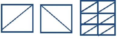
This method focuses on a topological feature of the 3D object which is the connectivity of mesh vertices. Therefore, embedding the watermark changes the topology of a model. The side effect of this is a change in geometry. Usually, working with topology is more robust for the watermarking, where the topology is redefined to encode one or more bits. One of the most famous examples of this type is encoding binary bits in triangulating a quadrilateral way [18]. Look to Figure 1.

Figure 1: Example of Topology Structure [18].

The wavelet transformation had been applied in the watermarking schema due to robustness measurements [6][17][24].

The pioneer works of watermarking 3D models were performed by Ohbuchi et al. [21], who introduced several schemes for watermarking polygonal models. One scheme embeds information using groups of four adjacent triangles, while another scheme proposed using ratios of tetrahedral volumes. The tetrahedral are formed by the three vertices of each face and a common vertex that is computed by averaging a few fixed mesh vertices. Moreover, a way of visually embedding information into polygonal mesh data is proposed by modifying the vertex coordinates, the vertex topology, or both. Ohbuchi et al. [22] also proposed a frequency domain approach to watermark 3D shapes, where the mesh is segmented first into some patches, and then for each patch, a spectral analysis is conducted, and the watermark information is finally embedded into the frequency domain at the modulation step.

The approach of Guillaume [10] is quite different; Guillaume presented a digital watermark embedded on 3D compressed meshes based on a subdivision surface, which chooses a 3D object segmented into surface patches as a target, and then hides the watermark in the compressed object.

Praun [27] provided a robust watermarking scheme suitable for proving ownership claims on triangle meshes representing surfaces in a 3D model by converting the original triangle mesh into a multiresolution format, consisting of a coarse base mesh and a sequence of refinement operations. Next, a scalar basis function is defined over its corresponding neighborhood in the original mesh. A watermark is then inserted as follows: each basis function is multiplied by a coefficient, and added to the 3D coordinates of the mesh vertices. Each basis function has a scalar effect at each vertex and a global displacement

direction, where this process is applied as a matrix multiplication for each of the three spatial coordinates x, y, and z.

In the 3D model represented as a cloud of vertices and a list of corresponding edges, Kundur [27] provided a new method based on finding and synchronizing particular areas used to embed the message by using data hiding that relies on modifying the topology of the edges in a chosen area. A wavelet-based multiresolution analysis is used for polygonal models proposed by Wan-Hyun Cho [33]. First, generate the simple mesh model and wavelet coefficient vectors by applying a multiresolution analysis to a given mesh model. Then, watermark embedding is processed by perturbing the vertex of chosen mesh at a low resolution according to the order of norms of wavelet coefficient vectors using a look-up table. The watermark extraction procedure is to take binary digits from the embedded mesh using a look-up table and similarity test between the embedded watermark and the extracted one follows.

JIN Jian-qiu et al [15] proposed a robust watermarking for 3D mesh. The algorithm is based on spherical wavelet transformation, where the basic idea is to decompose the original mesh of details at different scales by using a spherical wavelet; the watermark is then embedded into the different levels of details. The embedding process includes: global sphere parameterization, spherical uniform sampling, spherical wavelet forward transformation, embedding watermark, spherical wavelet inverse transformation, and at last re-sampling the watermarked mesh to recover the topological connectivity of the original model.

Adrian G.Bors [5] also proposed a public watermarking algorithm that is applied on various 3D models and does not require the original object in the detection stage using a key to generate a binary code. A set of vertices and their neighborhoods are selected and ordered according to a minimized distortion visibility threshold. The embedding consists of local geometrical changes of the selected vertices according to the geometry of their neighborhoods.

The approach proposed in [2] which uses a new blind digital watermarking algorithm is based on discrete wavelet packet transformation and a Backpropagation (BP) Neural Network. Backpropagation is a common method of training artificial neural networks so as to minimize the objective function The contribution in this paper is to apply digital watermarking algorithm based on a spherical wavelet transform [13] applied to polygonal 3D mesh models. These polygonal 3D mesh models were compressed using a Multi Layer Feed Forward (MLFF) neural network [25][26][29][30]. The paper will combine geometric methods with topological methods in the watermarking algorithm.

The proposed robust watermarking algorithm should meet the following technical requirements:

1. Direct Embedding: The watermark should be directly embedded into the compressed geometry data or topology data of the polygonal model. 2. Invisible: The embedded watermark must be

perceptually invisible within the model and unnoticeable for the user.

small enough in order not to disturb the application use.

4. Robustness: The embedded watermark must be unchanged or difficult to be destroyed under the possible 3D geometric operations done on the 3D polygonal model.

5. Capacity: The amount of the watermark which can be embedded in the model is large enough to record the information needed for the application. 6. Efficient Space: A data embedding method should

be able to embed a non-trivial amount of information into model.

This paper is divided as the following:

 In section II, a brief background is given about the proposed compression methodology based on a Multi Layer Feed Forward (MLFF) neural network [25][26][29][30].

 In section III, the output from compression, which is a compressed 3D polygonal mesh model, will be the input for a proposed watermarking algorithm. The algorithm applies the watermark, which can be a secret key or image, in a spherical wavelet transformation for the compressed data set [13].

 In section IV, testing results will be presented on some 3D models [29][30] samples. The proposed watermarking algorithm will be evaluated against various types of attacks [13].

 In section V, we present our conclusion. The experimental results show that the proposed watermark algorithm on compressed 3D objects:

1. Is a very efficient and robust. Moreover, it is proved to reduce the processing time. 2. Allow the embedding of the watermark

into the model without much increase on the model size.

2.

3D OBJECT COMPRESSION

ALGORITHM

neural network employed in this paper is a multilayer feed-forward neural network (MLFF) [25][26][29][30], which provides lossy compression. The neural network tool used for this algorithm is the Mathworks tool (Neural Network Toolbox’s with Multi-layer Feed Forward Architecture). MLFF is a well known neural model, which consists of an input layer, one or several hidden layers and an output layer. All nodes are fully connected. The neurons in the feed- forward neural network are generally grouped into layers. Signals flow in one direction from the input layer to the next, but not within the same layer. An essential factor of successes of the neural networks depends on the training network. Among the several learning algorithms available, back-propagation has been the most popular and most widely implemented.

The object has been created manually (modeling them using Autodesk Maya 2008); and before entering the data in MLFF. Pre-processing should be applied on the data [29][30]. The following sub-sections will briefly explain the steps of the compression [25][26][29][30].

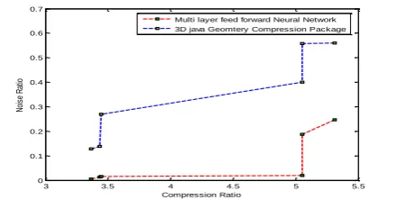
Figure 2 shows the difference between the MLFF neural network algorithm employed in this paper and the Java 3D geometry compression package.

Figure 2: Comparing between the MLFF compression algorithm and 3D Java geometry compression package

[29][30].

2.1 The Pre-Process Data Set

Before the inputs are presented to the MLFF, the data should be pre-processed. Accuracy of the outputs of the neural network depends on the data pre-processing step.

The following are the steps that should be done in the data pre-processing stage:

 Normalization

 Extract main features of the dataset

The supervised learning problem is divided into parametric and nonparametric models. The problem here lies in the nonparametric model because there is no prior knowledge of the form of the function being estimated. Therefore, it is required to use a neural network that could be trained using different models samples. This type of neural learning is called learn by example [29][30]. The learning process will be performed by a learning algorithm. The objective of this algorithm is to change the synaptic weight of the network to attain a desired design objective, which is the compressed object. Once the network has been trained, it is capable of generalization [29][30].

2.2 The Structure of the MLFF Neural

Network

The neural network structure contains an input layer, one hidden layer, and an output layer; all nodes are fully connected. The network takes x, y and z coordinates of vertices as input; the activation function is a sigmoid logistic function with a learning rate of 0.9 [29][30].

A sigmoid logistic function, also known as a logistic function, is given by the relationship [29][30]:

where β is a slope parameter. The sigmoid has the property of being similar to the step function, but with the addition of a region of uncertainty. Sigmoid functions in this respect are very similar to the input-output relationships of biological neurons, although not exactly the same. Below is the graph of a sigmoid function. Sigmoid functions are also prized because their derivatives are easy to calculate, which is helpful for calculating the weight updates in certain training algorithms. The derivative is given by [29][30]:

3 3.5 4 4.5 5 5.5

0 0.1 0.2 0.3 0.4 0.5 0.6 0.7

Compression Ratio

N

oi

se

R

at

io

The number of neurons in the input layer is 4, where the first three input vectors are the x, y and z vertices coordinates, and the fourth input is the maximum face ratio which indicates that the maximum face must remain as it is. The number of neurons in the hidden layer is between 3 and 4. The compression process overall depends on the hidden layer, so the number of neurons in the hidden layer should be absolutely less than the number of neurons in the input layer to do the compression. For higher accuracy, the number of neurons in the hidden layer should be increased, but this reduces the compression process. A two-layer feed-forward network with sigmoid hidden neurons and linear output neurons can fit multi-dimensional mapping problems arbitrarily well, given consistent data and enough neurons in its hidden layer [29][30]. Figure 3 displays the neural network structure with a given 3D model object sample for input object and target object.

2.3 The Training Samples

There are three main aims for the geometry compression technique; efficient rendering, progressive transmission, and maximum compression to save disk space [8]. Geometry compression using the Java 3D package can achieve lossy compression ratios between 10:6 to one object, depending on the original representation format and the desired quality of the final level. Decompression is the reverse of this process. The improvement in this package by adding optimization compression makes the lossy in detail of the 3D object much smaller.

Figure 3: One hidden layer Feed Forward Neural Network Structure [29][30].

The geometry compression algorithm steps for the Java 3D package are as follows [8]:

1. Input explicit bag of triangles to be compressed, along with quantization thresholds for positions, normals, and colors.

2. Topologically analyze connectivity, mark hard edges in normals and/or color.

3. Create vertex traversal order & mesh buffer references.

4. Histogram position, normal, and color deltas. 5. Assign variable length Huffman tag codes for deltas,

based on histograms, separately for positions, normals and colors.

6. Generate binary output stream by first outputting Huffman table initializations, then traversing the vertices in order, outputting appropriate tag and delta for all values.

Also, there are some definitions that have been added to identify the critical vertices, so that removing those critical vertices can be controlled such that the number of vertices remains correspondent to the edges which are never used by the compression algorithm. The following are the definitions of those vertices depending on invariant vertex identification that is provided by [20]:

1. Boundaryvertices of the 3D model are the vertices that cannot be used by the compression algorithms because these are critical vertices. These are defined as vertices which influence the shape of the 3D model.

2. Neighboring vertices to split a vertex will never be used by the compression algorithms.

3. Vertices of edges which do not form a simple triangle cannot be collapsed. That can be calculated from the data of 3D models by storing all the vertices and faces according to the label of vertices, and then checking every two consecutive faces. If any two consecutive triangles have two of its vertices in common, so that two vertices form a complex triangle. In this way, this pair of vertices cannot be used by the compression algorithm. The complexity of invariant vertex selection is analyzed as follows according to [7]:

1. The complexity of selecting boundary vertices of the 3D object by computing convex hull takes O(n log n) using a quick hull algorithm [9].

2. The neighboring vertices, which are computed after each refinement, has to be split. These set of vertices vary according to the compression scheme used If p is the number of split vertices in a refinement, and d is the maximum degree for a vertex, then the complexity for processing these set of vertices is O(p*d).

3. Computing the vertices of edges which are not simple triangles. First, sort all the faces according to the label of vertices which takes O(n log n). Then, checking between two consecutive faces takes O(n) time.

Therefore, the overall worst time complexity of the invariant vertex selection algorithm is :

Where T (n) is time complexity and n is the number of vertices.

The overall complexity of remesh algorithm using Java 3D geometry compression in addition to invariant vertex selection algorithm is as follows[29][30]:

1. The invariant vertex selection algorithm complexity (see equation 2.1) is:

T(n) = 3nlog n + n = O(n log n), 2. The remesh algorithm complexity is:

T (n) =15n+4 = O(n). (2.2) 3. from equations (2.1) and (2.2):

T (n) = (3n log n +n) * (15n + 4), T (n) = 45n2 _{log n +15 n}2 _{+12 n log n +4n} = O(n2 log n) (2.3) Where T (n) is time complexity and n is the number of vertices. Therefore, O (n2 log n) is the overall worst time complexity of the remesh algorithm in addition to invariant vertex selection.

Theorem 1 [30]: The overall worst time complexity of the compression algorithm using the proposed MLFF neural network is O(n3).

Proof:

Equation (2.1) is the worst time complexity for invariant vertex selection algorithm. Equation (2.2) is the worst time complexity for remesh algorithm. Equation (2.3) is the worst time complexity for remesh algorithm in addition to identifying for invariant vertex.

The Worst time complexity for pre- process data set (i.e. section 2.1) is [29][30]

T (n) =10n (2.4)

The worst time complexity for MLFF neural network given in this paper is [25][26][29]

T (n) =n3 (2.5)

From all of the above, equation (2.1), equation (2.2), equation (2.3), equation (2.4) and equation (2.5) :

T (n) = O (n3_).

Where T(n) is overall time complexity and n is the number of vertices.

2.4 The Results

The network trains 1000 times with the training set until the Mean Square Error (MSE) is small; say less than a given

, this MSE is the difference between the output objects and desired objects, and is given by:

(2.6) Where X are the coordination vertices (3D point) in original mesh, X' are the coordination vertices (3D point) in compressed mesh, N denotes the number of rows and M the number of columns in the array of vertices coordinated, respectively. Training automatically stops when generalization stops improving, as indicated by an increase in the Mean Square Error (MSE) of the validation samples [30].

The network will be trained with a gradient-descent back propagation algorithm with adaptive learning rate. Training time for each model takes approximately 2 hours and 30 minutes; for all the ten models takes 25 hours and 12 minutes [30]. In another set of experiments, training time for each model takes approximately 5 hours and 4 minutes. For all the ten models, it takes 55 hours and 40 minutes [29].

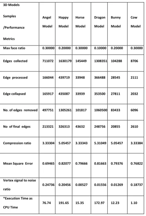
Table 2.1 shows the results achieved by the proposed algorithm for some models. Angel Model[29], Happy Model[29], Horse Model[29][30], Dragon Model[29], Bunny Model[29][30], and Cow Model[29][30].

They entered to MLFF neural, where:

Compression Ratio =

Signal to Noise Ratio =





N

i

N

1

[(X'– X)2 _{+ (Y'– Y)}2_{+(Z'– Z)}2_]

where N denotes the number of vertices, X', Y' and Z' are coordinates in compressed 3D object and X, Y and Z are the coordinates in the original object.

Obviously, the number of neurons in the input layer is 4, hence, the total size of the object on Disk = nf *ns *4*3, where nf denotes the number of faces, ns denotes the number of vertices. Denote that each face has three vertices and the number of neurons in the input layer is 4. Size will be in byte. See figure 4 for an example of a model before and after compression.

By using MLFF neural network algorithm, the performance of the compression increases. The compression ratio is between 5.3 and 3.3 of the original object. The noise ratio depends on the MSE (error function), given equation (2.6), which provides minimum noise for the visual eye [29][30].

3.

WATERMARKING ALGORITHM

FOR COMPRESSED 3D OBJECT

The output result from the compression algorithm mentioned in the previous section, which is the compressed 3D model, will be the input for the watermarking algorithm proposed in this section. The proposed watermarking algorithm is based on a spherical wavelet transformation which is considered among the most robust watermarking methods [6][17][24]. The watermarking algorithm in this paper is based on the method in [13], which performs the efficient spherical wavelet function, depending on the spherical wavelet presented in [31]. The following sections will explain how the proposed algorithm should embed and extract the Watermark in the

compressed 3D mesh model.

3.1 Generate the Sphere Coordinate for

Each Vertex in 3D Mesh using spherical

parameterization

3.1.1 Construct a harmonics function on the

Sphere and perform spherical harmonic

transformation

It is popular to represent a 3D shape with functions

grid of size n x n of angles of elevation (0≤ ≤π), and azimuth (0≤ ≤2π).

Spherical harmonic function represents a data set on the sphere. The function used for this representation is spherical harmonics that helps in making the multi-resolution representation of the 3D mesh. Any point on the unit sphere can be denoted as follows:

P = (cos sin , sin sin , cos ), where (0≤ ≤π) and (0≤ ≤2π) denote the angles of longitude and latitude respectively. The spherical shape function is defined on the unit sphere and the expansion of in spherical harmonics is defined to be [19]:

(3.1) Where the normalized spherical harmonics

_are defined respectively by:

(3.2) And

(3.3) where

= , and

is the associated Legendre polynomial of and

By Rodrigues’ formula :

where

, m ={-l, -l+1, …,l-1,l}

3.1.2 Perform a Spherical Parameterization for

the 3D Mesh

Parameterization is crucial to many applications such as texture mapping, morphing and geometric signal processing.

Spherical parameterization is mapping a mesh into a sphere such that the 3D model can be defined as spherical signals. This step requires that the mesh is homeomorphic to sphere [14]. Several methods were developed for parameterization over the unit sphere [1][14][28][34]. We use the algorithm developed in [13][34].

The parameterization of a triangle mesh onto the sphere means assigning a 3D position on the unit to each of the mesh vertices. The topological sphere for the 3D object is a close manifold genus mesh that means embedding its connectivity graph on the sphere to get a spherical parameterization of the original mesh.

Table 2.1: Compression result of the proposed MLFF neural network [29][30]. (*CPU Time returns the total CPU time (in seconds) used by MATLAB® application from the time it was started. This number can overflow

the internal representation and wrap around.)

According to [19], the basis mesh is transformed into a spherical mesh using centric. Therefore, a sequence of successive vertex split operations and the corresponding local parameterization of the deleted vertices on the spherical mesh have been applied. As illustrated in figure 5, the method described in [13] involves the following steps that explain how spherical parameterization information is generated for the 3D mesh:

1. Generating a progressive mesh representation with local parameterization information based on equations (3.1), (3.2) and (3.3). Edge collapse operation is iteratively performed until the mesh is simplified into a convex polyhedron. For each edge collapse, the two decimated vertices are parameterized over the resultant simplified mesh. 2. Start with the initial spherical mesh yielded by

projecting the base mesh recorded in the previous step onto the unit sphere. The sequence of vertex split operations is performed progressively. For each vertex split, the two split vertices are positioned on the unit sphere using the recorded connectivity and local parameterization information. The procedure of edge collapse with local parameterization is in Figure 6 [13].

3. Computing the subdivision of each triangle into 4 smaller triangles in 3D mesh, and then project on the sphere whose radius is one unit.

Generally speaking, the steps commonly used to compare 3D shapes are [16]: Normalization, Parameterization, Spherical Harmonic Transform (SHT), and Shape descriptors.

Figure 7 shows the samples for applying section 3.1 on 3D mesh model. The output of section 3.1 will be the input of next section 3.2.

3.2 Generate the Spherical Wavelet

Transformation

Wavelets have been proved to be powerful bases for use in signal processing based on the fact that they only require a small number of coefficients to represent general functions and large data sets. Due to local support in both the spatial domain and the frequency domain, which are suited for spare approximation of function, the spherical wavelet transform is chosen in this work. In fact, wavelets are basis functions which represent a given function at multiple levels of detail. Due to their local support in both spatial domain and frequency domain, they are suited for sparse approximations of functions. We adopt the spherical wavelet proposed in [31]. In particular, the butterfly wavelet transformation is selected. The following is a brief description about the wavelet transformation in general, and later the butterfly wavelet transformation in particular.

The general wavelet transformation of a function is constructed as follows [31]:

Analysis: (forward transform)

(3.4) This represents the scaling function coefficient, fine to coarse.

(3.5) This represents wavelet coefficient, fine to coarse On the other hand, the inverse wavelet transformation [31]:

Synthesis: (backward transform)

(3.6) This represents the scaling function coefficient, coarse to fine. In equations (3.5) and (3.6), n,• and ,• are the

approximation and wavelet coefficients of the function at resolution j, respectively. The decomposition filters ĥ, ĝ, and the synthesis filters h, g corresponds to the spherical wavelet basis functions. The forward transform is performed recursively starting from the shape function  = n,• at the finest resolution n to get n,• and ,• at level j, j=n-1,…,0. The

coarsest approximation n-i,• is obtained after i iterations (0 < i ≤ n). In other words, when n,• (n is finest resolution level) is given, we can recursively perform the above analysis process (forward transform) to get ,• the wavelet coefficients at the current level, and the coarsest approximation part n-i,• after performing the decomposition i

3D Models

Samples

/Performance

Metrics

Angel

Model Happy

Model Horse

Model Dragon

Model Bunny

Model Cow

Model

Max face ratio 0.30000 0.20000 0.30000 0.10000 0.20000 0.30000

Edges collected 711072 1630179 145449 1308351 104288 8706

Edge processed 166044 439719 33948 366488 28545 2111

Edge collapsed 165917 435087 33939 353500 27811 2032

No. of edges removed 497751 1305261 101817 1060500 83433 6096

No of final edges 213321 326313 43632 248756 20855 2610

Compression ratio 3.33304 5.05457 3.33343 5.31049 5.05457 3.33384

Mean Square Error 0.69465 0.82077 0.79666 0.81663 0.79376 0.76822

Vertex signal to noise

ratio

0.24736 0.20456 0.00527 0.01556 0.01269 0.18737

*Execution Time as

CPU Time

times [13]. Similarly, if we have n-i,• and ,• (j=n−i, n−i+1, ..., n−1), we can perform the synthesis process (inverse transform) recursively to get the n,• Different h, ĥ, g, ĝ denote different wavelet basis function. In Euclidean space we have hj, k, l =hi-2k (the same with g, ĝ), but in general manifold they are dependent on scale and position. The abstract sets M(j) and K(j) are index sets on the sphere such that

, and K(n) = K is the index set at the finest resolution.

The mesh including dashed edges in the figure 8 is assumed as resolution j+1 level. Here K(j) denotes the point set of the intersection points of the solid lines and M(j) denotes the set of the intersection points of the dash lines. We will compute the j and approximation part and detailed part, by single decomposition in the neighborhood of m [13].

The work done in [13] was based on linear and linear-lifting transformation methods, where in linear transformation, the scaling coefficients (approximation part) are sub-sampled and kept unchanged. This basic inter-polatory form uses the stencil k K = {v1,v2} for analysis and synthesis:

(3.7)

(3.8) respectively.

Note that this stencil does properly account for the geometry provided that the m sites at level j+1 have equal geodetic distance from the {v1,v2} sites on their parent edge. Linear lifting update the scaling coefficients by using the wavelet coefficients of linear wavelet transform to assure that the wavelet has at least one vanishing moment sj,v1,m = sj,v2,m = 1/2. In this work the Butterfly transformation [31] is used to decompose the geometric signal of the approximation and detailed parts, and uses all immediate neighbors (all the sites km = {v1,v2, f1,f2,e1,e2,e3,e4}. Where sv1=sv2= , sf1=sf2= and se1=se2=se3=se4= - ) in construction of the smooth mesh.

Analysis: (Butterfly Transformation)

(3.9)

(3.10)

Synthesis: (Butterfly Transformation)

(3.11)

(3.12)

Figure 5: Global spherical parameterization [13]

Figure 6: Edge collapse with local parameterization [13]

The butterfly transformation is considered to take more time than a linear transformation, but because the work is on a compressed domain this makes the butterfly and linear close in time consumption. However, the butterfly is supposed to be more robust as regards the watermarking algorithm; in this work the level wavelet decomposition will be to 3 levels (see figure 9).

Figure 8: Neighbors used in spherical wavelet transformation [13].

The following sections will explain how the proposed algorithm should embed and extract the Watermark in the compressed 3D mesh model.

3.3 Embedding Watermark

[11]

3.3.1 Generation Watermark and its Capacity

A watermark can be a secret key or image. This algorithm is adopted to embed a watermark as a secret key or image. Embedding a watermark by these two ways should be sequences of binary bits, which means that by the secret key case (all characters and numbers) should be converted to a sequence of binary bits; and in the case of image, the image should be converted to a gray scale level in order to be as a sequence of binary bits. However, in all experimental results that have been displayed in this paper, just the image method was used because it is more complex than the secret key, and this assures coverage for the entire model.

Capacity of Watermark means the amount of information embedded in a 3D object; this amount should be closely related to the complexity of the object (number of vertices, number of faces). It is assumed that the data capacity of a watermark should be not more than the complexity of the 3D object, depending on the number of vertices. Dependent on choosing the watermark as an image, the logo image shouldn’t be more 125*125 pixels (which was observed from experiments) and then converted to binary (gray scale), which produced 16384 bits ready to embed into the 3D object.

3.3.2

Watermark Embedding

The watermark embedding is done by the following equation:

(3.13)

where is the ith vertex of M′ after the watermark is embedded and belongs to band j. On the other hand, is the set of all vertices of M and belong to band j. w is the

watermark (logo image for example), and F(•) is a function to compute the weight of the embedding intensity, which is related with the band j. Here is used to control the global intensity of the watermark and is only related with band j. In our implementation, the function F is defined by [13]:

(3.14)

3.4 Extracting the Watermark

In order to extract the watermark from a 3D model the following steps have been applied:

Figure 9: The samples before and after applying the spherical wavelet transformation. The colored vertices are

3.4.1 Mesh Registration

The mesh registration used here is based on the ICP (Iterative Closest Point) algorithm [4]. It was applied on the watermarked mesh as follows:

Input: The point set P with Np points from the data shape and the model shape M (section 3.2). The data set is initialized. The registration vectors are defined relative to the initial data set.

Output: The final registration vectors output represents the complete transformation.

Process: The following four steps are applied until convergence within a tolerance

1. Compute the closest points of the Squared Euclidian distances ,

2. Compute the registration (rotation and translation), 3. Apply the registration,

4. Terminate the iteration when the change in Mean Square Error (MSE) equation (2.6) falls below a preset threshold .

3.4.2 Spherical Wavelet Forward Transformation

After producing the mesh registration, the spherical wavelet forward transformation is applied on two meshes

1. The registration mesh

2. The compressed mesh (i.e. the original mesh before applying the watermarking algorithm)

Compare the results of the meshes in order to extract the watermark image as a sequence of binary digits (see sub-section 3.3.1).

4. EXPERIMENTAL RESULTS AND

EVALUATIONS AGAINST ATTACKS

4.1 Performance evaluation

This section presents the evaluation of the proposed watermarking algorithm. There are two performance metrics, which will be discussed below.

4.1.1 Sampling and precision control

The visual impact of the watermarking on the protected 3D object should be as limited as possible to measure the effect of the embedded watermark on 3D objects.

In this paper, Hausdorff distance d is used to quantify the maximum geometric error. Generally speaking, the Hausdorff distance d is a measure defined between two point sets.

In section 3.1, the geometrical signal on the unit sphere has been obtained. In order to perform spherical wavelet transform over the geometrical signal, the signals should be sampled regularly over the sphere. As illustrated in figure 10, we first perform recursive 1-split-to-4 subdivision of the tetrahedral base shape as used by [31], and then we sample the signals at the vertices of the subdivision spherical mesh. In practice, we wish that the

generated regular mesh approximates the original mesh with a given tolerance

Let M be the original mesh and SM is the sampled mesh. We perform inverse sampling on SM to get mesh M′. The inverse sampling will be executed until the following equation is satisfied [13]:

where is a user-specified error threshold, and are vertices on M and M′ respectively.

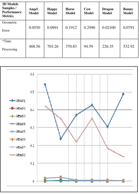
4.1.2 Processing Time

For this watermarking algorithm, most of the time consumed was spent on calculating coefficients by spherical wavelet transformation; the embedded watermark and extracted watermark don’t take a lot of time compared with wavelet transformation. There is no mathematical way to calculate the time processing here but by experimental results shown in table 2.1, it can be noticed that time processing increases according to an increasing number of vertices. Table 4.1 shows the results that have been achieved by applying the watermarking algorithm in this paper on the six models [29][30].

4.2 Testing

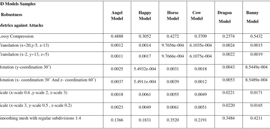
For testing the watermarking algorithm implemented in this paper, the following attacks were chosen to attack 3D models samples [29][30]:

1. Translation (x+20,y-5,z-13). 2. Translation (x-2, y+13, z+5). 3. Rotation (y- coordination 30˚).

4. Rotation (x-coordination 30˚ and z-coordination 60˚). 5. Scale (x-scale 0.6,y-scale 2, z-scale 3).

6. Scale (x-scale 3, y-scale 0.5, z-scale 0.2).

7. Smoothing mesh as noise filtering with regular subdivisions 1:4.

8. Lossy compression provided by [10], (look to figure 11). To measure the robustness of the watermarking algorithm, the following measurements were used:

1- The Bit Error Rate (BER) is used, see Equation (4.2). The BER is a rate that measures the errors that appear after the 3D model is attacked (the ratio of number of destroyed bits to the total bit length in the extracted watermark).

(4.2) where is the sequence of binary bits embedded into the 3D model before being distributed over the Internet and attacked; is the sequence of binary bits that are extracted from the 3D model after being attacked; ⊕is an

(Exclusive Or) operation that leads to a sequence of ones in the positions that had errors;Counterrors is a counter that holds how

2- The Survival Rate (SR) is the rate of survival of a watermark under attack formations.

SR = 1-BER (4.3) Table 4.2 shows the measurements of robustness that are achieved by applying the watermarking algorithm in this paper on the models of [29][30] using BER. Table 4.3 shows the measurements of robustness achieved by applying the watermarking algorithm in [13] also using BER. From the results that appear in Tables 4.2 and 4.3 it had been confirmed that applying a watermarking algorithm on a compressed domain is more robust than applying a watermarking algorithm on a normal domain. Figure 12 and Figure 13 show a comparison between the performed work in this paper and the work in [13] from the robustness of two watermarking algorithms against the attacks on the models of [29][30]. This clearly shows that the performance from the BER of proposed watermarking algorithm is better in most types of attacks than the algorithm in paper [13].

Figure 10: Spherical meshes subdivision. The subdivided meshes are used for sampling [31]

Figure 11: The Happy Model Before and After Compression attack [29].

Table 4.1: Performance measurement of the watermarking algorithm in this work (*CPU Time returns the total CPU time (in seconds) used by MATLAB® application from the time it was started. This number can overflow the internal

representation and wrap around.)

Figure 12: Experimental result for the work proposed in [13]

Figure 13: Experimental result for the work in this paper

3D Models Samples / Performance Metrics

Angel Model

Happy Model

Horse Model

Cow Model

Dragon Model

Bunny Model

Geometric

Error 0.0550 0.0991 0.1912 0.2990 0.02100 0.0791

*Time

Table 4.2: Robustness measurement results of BER for a watermarking algorithm in this paper.

Table 4.3: Robustness measurement results of BER for the algorithm in paper [13].

5. CONCLUSIONS

A compression algorithm using an MLFF neural network that produces a compressed 3D model (with a compression ratio that reaches 5.5) reduces the size of the 3D model with minimum loss of details and vertex signal to noise ratio. This is noticed experimentally by applying the proposed algorithm on different 3D models samples [29][30]. The MLFF neural network as an AI tool played an important role in the

performance of the compression algorithm making the algorithm’s performance better than the 3D compression geometry proposed in [31].

The methodology of applying a watermark on a 3D model after compression, on a compressed domain, is proved to reduce the processing time of the watermarking algorithm, in addition to allowing the embedding of the watermark into the model without much increase on model size, compared to the

3D Models Samples

/ Robustness

Metrics against Attacks

Angel Model

Happy Model

Horse Model

Cow Model

Dragon

Model

Bunny

Model

Lossy Compression 0.0291 0.0535 0.0945 0.1764 0.0665 0.1160

Translation (x+20,y-5, z-13) 0.0018 4.2725e-004 0.0015 2.4414e-004 9.4604e-004 5.4932e-004 Translation (x-2, y+13, z+5) _{0.0011 4.2705e-004 0.0035 2.4454e-004} 9.4613e-004 5.4902e-004

Rotation (y-coordination 30˚) _{0.0020 9.7656e-004 0.0013 3.0518e-004} 6.7139e-004 0.0068

Rotation (x- coordination 30˚ And z- coordination 60˚) _{0.0026 9.7436e-004 0.0025 3.0508e-004} 6.7139e-004 0.0040

Scale (x-scale 0.6 ,y-scale 2, z-scale 3) _{8.2393e-004 4.5746e-004 1.5279e-004 7.0180e-004} 5.1890e-004 0.0042

Scale (x-scale 3, y-scale 0.5 , z-scale 0.2) _{8.2397e-004 4.5776e-004 1.5259e-004 7.0190e-004} 5.1880e-004 0.0012

Smoothing mesh with regular subdivisions 1:4 _{0.0183 0.0237 0.0243 0.0304} 0.0245 0.0400

3D Models Samples

/ Robustness

Metrics against Attacks

Angel Model

Happy Model

Horse Model

Cow Model

Dragon

Model

Bunny

Model

Lossy Compression 0.4888 0.3052 0.4272 0.3709 0.2374 0.5432

Translation (x+20,y-5, z-13) 0.0012 0.0014 9.7656e-004 6.1035e-004 0.0024 0.0015

Translation (x-2, y+13, z+5) _{0.0011 0.0017 9.7666e-004 6.1075e-004} 0.0022 0.0019

Rotation (y-coordination 30˚) _{0.0025 5.4932e-004 0.0031 0.0018} 0.0043 8.5449e-004

Rotation (x- coordination 30˚ And z- coordination 60˚) _{0.0037 5.4911e-004 0.0039 0.0012} 0.0053 8.5489e-004

Scale (x-scale 0.6 ,y-scale 2, z-scale 3) _{0.0018 0.0061 0.0055 0.0049} 0.0221 0.0171

Scale (x-scale 3, y-scale 0.5 , z-scale 0.2) _{0.0023 0.0049 0.0061 0.0051} 0.0220 0.0165

original model before compression. Implementing the watermarking algorithm is based on a spherical wavelet as a butterfly transformation method for vertex bases wavelet coefficients. The experimental results and evaluation against attacks shows that watermarking algorithm proposed in this paper met the technical requirements of robustness that mentioned earlier in this paper.

6. REFERENCES

[1] Alexa, M., "Recent a d v a n c e s in mesh m o r p h i n g " , Computer Graphics Forum, 21(2):173-196 (2002). [2] Baoming Q., Pulin Z., and Qiao K., "A Digital

Watermarking Algorithm Based on Wavelet Packet Transform and BP Neural Network", Seventh International Conference on Computational Intelligence and Security (2011). DOI 10.1109/CIS.2011.117 [3] Benedens O., "Geometry-Based Watermarking of 3D

Models", IEEE Computer Graphics and Applications 19(1), 46–55 (1999).

[4] Besl P. and McKay N., "A Method for Registration of 3-D Shapes", IEEE Trans. on Pat. Anal. and Mach. Int., Vol. 14, N. 2, pp. 239-256 (1992).

[5] Bors A., "Watermarking mesh-based representations of 3-D objects using local moments" , IEEE Transactions on Image Processing 15(3), 687–701 (2006).

[6] Chen S-T, Huang H-N, Hsu C-Y, Tseng K-K, Wu C., and Pan J-S, "Wavelet-Based Entropy for Digital Audio Watermarking", Seventh International Conference on Intelligent Information Hiding and Multimedia Signal Processing (2011).DOI 10.1109/IIHMSP.2011.39 [7] Cox I, Miller M., Bloom J., "Digital Watermarking:

Principle & Practice", ( The Morgan Series in Multimedia and Information Systems), ISBN-1558607145 (2001).

[8] Deering M. "Geometry compression", ACM SIGGRAPH, pp. 13–20 (1995).

[9] Fornaro C. and Sanna A., "Public Key Watermarking for authentction of CSG models", Computer Aided Design, 32(12), 727-735 (2000).

[10]Guillaume L., Denis F., Dupont F., "Subdivision surface watermarking. Computers & Graphics", 31(3): 480-492 (2007).

[11]Isenburg M. and Snoeyink J., "Face fixer compressing polygon meshes with properties", ACM Siggraph Conference Proc, pp. 263-270 (2001).

[12]Jianhong S, Junsheng L., and Zhiyong L., "An Improved Algorithm of Digital Watermarking Based on Wavelet Transform", World Congress on Computer Science and Information Engineering (2009). DOI 10.1109/CSIE.2009.150

[13]JQ J., MY D., HJ B. and QS P., "Watermarking on 3D mesh based on spherical wavelet transform", Journal of Zhejiang University SCIENCE pp. 251–258 (2004). [14]Kent, J.R., Carlson, W.E., and Parent, R.E., "Shape

Transformation for Polyhedral Objects", SIGGRAPH, Computer Graphics Proceedings, Annual Conference Series, ACM, p.47-54 (1992).

[15]Kundur D. and Hatzinakos D., "Robust digital image watermarking method using wavelet-based fusion", Proc. of IEEE Int. Conf. on Image Processing, Vol.1, pp.544-547 (1997).

[16]Laga H; Nakajima M; and Chihara, K. H., "Discriminative spherical wavelet features for content-based 3D model retrieval", International Journal of shape modeling (2007).

[17]Li Y., Gou W. and Li B., "A new digital watermark algorithm based on the DWT and SVD", 10th International Symposium on Distributed Computing and Applications to Business, Engineering and Science (2011). DOI 10.1109/DCABES.2011.7

[18]Li L, Pan ZG, Sun SS and Wu XL "A private and lossless digital image watermarking system. In: Proceedings of second international conference on image and graphics, Hefei, China, SPIE, p. 365–70 (2002). [19]Li, L., Zhang, D., Pan, Z., Shi, J., Zhou, K. and Ye, K.,

"Watermarking 3D Mesh by Spherical Parameterization. Computers and Graphics", 28(6), 981–989 (2004). [20]Maheshwari P., Agarwal P., and Prabhakaran B.,

"Progressive compression invariant semi-fragile Watermarks for 3D meshes", in Proceedings of ACM Multimedia and Security Workshop (2007) (MM&Sec 2007), Dallas, TX , USA , pp. 245-25, (2007).

[21]Ohbuchi R., Masuda H. and Aono M., "Watermarking multiple object types in three-dimensional models", Multimedia and Security Workshop at ACM Multimedia, Bristol, UK (1998).

[22]Ohbuchi R., Mukaiyama A. and Takahashi J., "Watermarking a 3D shape model defined as a point set", International Conference on Cyberworlds (2004).

[23]Ohbuchi R. , Nakazawa M. and Takei T., "Retrieving 3D shapes based on their appearance", ACM SIGMM Workshop on Multimedia Information Retrieval, Berkeley, California, pp. 39–46 (2003).

[24]Okagaki K., and Takahashi K., "Robustness Evaluation of Digital Watermarking Based on Discrete Wavelet Transform", Sixth International Conference on Intelligent Information Hiding and Multimedia Signal Processing (2010). DOI 10.1109/IIHMSP.2010.36

[25]Piperakis E., "Transformations on 3D Objects Represented with Neural Networks", IEEE, Proceedings of the Third International Conference on 3-D Imaging and Modeling, (2001).

[26]Piperakis E., and Kumazawa I, "3D Polygon Mesh Compression with Multi Layer Feed Forward Neural Networks", Systemics, Cybernetics, and Informatics , Volume 1, Number 3, (2002).

[27]Praun E., Hoppe H. and Finkelstein A., "Robust mesh watermarking", ACM SIGGRAPH, Los Angeles, California, pp. 49–56 (1999).

[28]Quicken, M., Brechbühler, C., Hug, J., Blattmann, H., and Székely, G., "Parameterization of Closed Surfaces for Parametric Surface Description", CVPR, p.354-360 (2000).

Thesis in Computer Science, Faculty of Graduate Studies Al-Balqa' Applied University, Jordan, August, (2009). [30]Rumman N. A., El-Seoud S. A., Khatatneh K. F., and

Gutl C, "Geometry Compression for 3D Polygonal Models using a Neural Network", International Journal

of Computer Applications (0975-8887)-Volume 1-No. 20, (2010).

[31]Schröder P. and Sweldens W., "Spherical wavelets: Efficiently representing functions on the sphere", ACM SIGGRAPH 95, 161-172 (1995).

[32]Shusen S., Li Li P. Z and Jiaoying S., "Robust 3D model watermarking against geometric transformation", CAD/CG’2003, October 29–31, Macao. China ,p. 87–92 (2003).

[33]Yeo B., Yeung M., "Watermarking 3-D Objects for Variations", IEEE Computer Graphics and Application, Vol. 19,36–45 (1999).