Testing the Long Memory Features in Return and Volatility of NSE Index

http://dx.doi.org/10.4236/tel.2015.53050

Testing the Long-Memory Features in

Return and Volatility of NSE Index

Naseem Ahamed1_{, Mamoni Kalita}2_{, Aviral Kumar Tiwari}1 1_{IBS Hyderabad, IFHE, Hyderabad, India}

2_{ICFAI University,Agartala, India}

Email: [email protected]

Received 21 May 2015; accepted 26 June 2015; published 29 June 2015

Copyright © 2015 by authors and Scientific Research Publishing Inc.

This work is licensed under the Creative Commons Attribution International License (CC BY). http://creativecommons.org/licenses/by/4.0/

Abstract

Long-term memory of stock markets is a topic that has not received its due attention from aca-demics. Posting the assertion made by Fama, 1970 [1] about markets being efficient, no one can consistently outrun it for a longer duration. Handful of papers checked the efficiency in emerging markets to see if the efficiency proposition held true. Furthering the literature in this study we test for the long-term memory of National Stock Exchange (NSE) index, Nifty and NSE_500 which are a collection of 50 and 500 listed firms respectively in India. The duration of the data for study is roughly eight years over the period from 2006-06-29 to 2012-09-13, a total of 1545 observa-tions. We observe that long-term memory does exist in the context of Indian stock market index.

Keywords

NSE Index, Volatility, Long-Memory, Stock Market

1. Introduction

the market and make speculative profit at the expense of others. All of these happen because of the lack of com-plete arbitrage of market information. Long-term memory hence intuitively is a characteristic of less developed financial market as opposed to an efficient one. Most of the previous studies found that emerging stock market countries are far from efficient due to the increase in the number of retail and institutional investors trading on stock markets. The different reactions in terms of their degree of information, interests and risk profiles, and reactions to news across different times are believed to be producing long memory in the stock return volatility. Earlier literatures on the strand of long memory and volatility are from diverse regions of the world like Ger-many, Malaysia etc. A few pertinent articles of Bilel, T. M. & S. Nadhem (2009) [2], Corhay, A., A. T. Rad, & J. P. Urbain (1995) [3], Gurgul, H., & T. Wójtowicz (2006) [4], Kang, S. H., Cheong, C. C. & Yoon, S. M. (2010) [5], Tan & Khan (2010) [6], Kang, S. H. & Yoon, S. M. (2007) [7], Kang, S. H. & Yoon, S. M. (2008) [8], Lo, A. W. (1991) [9] need to be mentioned. This study attempts to test if stock returns and volatility exhibit long memory in national stock exchange (NSE) price indices over the period from 2006-06-29 to 2012-09-13, a total of 1545 observations.

2. Methodology

In this section we briefly explain about Autoregressive Fractional Integrated Moving Average (ARFIMA) model, Fractional Integrated GARCH (FIGARCH) model and the Fractional Integrated Asymmetric Power ARCH (FIAPARCH) model.

2.1. Autoregressive Fractional Integrated Moving Average (ARFIMA) Model

Following the Granger and Joyeux (1980) [10], and Hosking (1981) [11], for the series xt, t=1,,T the ARFIMA(r, d, s) model may be expressed as follows:

( )(

L 1 L

)

d

(

x_t µ

)

( )

L ε_t

Ψ − − = Θ (1)

( )

~ 0,1 ,

t zt t zt

ε = σ (2)

where μ is conditional mean and εt is independent and identically distributed (i.i.d.) with a variance σ2, and L is the lag operator as denoted earlier.

( )

1 2 2

r r

L ψ L ψ L ψ L

Ψ = + + + and

( )

1 2 2

s s

L θL θ L θ L

Θ = + + + are the autoregressive (AR) and moving-average (MA) polynomials lie outside of unit cycles, respectively.

The process is said to be long memory at the long run as long as d > 0 in Equation (1). In particular, for

(

0, 0.5 ,

)

d∈ and d ≠ 0, the series is covariance stationary and mean reverting, with shocks disappearing in the long run; for d∈

(

0.5,1

)

, the series imply mean-reversion, however, it is not a covariance stationary process as there is no long run impact of an innovation on future values of the process. For d ≥ 1, the series is non-statio- narity and non-mean-reversion. On the contrary, the process is said to exhibit intermediate memory, for

(

0.5, 0

)

d∈ − .

2.2. Fractional Integrated GARCH (FIGARCH) Model

Similar research on the volatility has led to an extension of the ARFIMA representation in 2 t

ε , leading to the FIGARCH model. Baillie et al. (1996) [12] have extended the traditional GARCH model to capture the long memory component in the return’s volatility. The FIGARCH (p, ξ, q) model is given by

( )(

)

2

( )

(

2 2

)

1 _t 1 _{t t}

L L ξ L

φ − ε = + −ω _ β _ ε −σ

Or

( )

( )

( )(

)

2 2 2 2

1 1

t L t L t L L t

ξ

σ = +ω β σ + −_ β _ε −φ − ε

where

( )

1 2 2 ,

q q

L L L L

φ =φ +φ + + φ and

( )

1 2 2 .

p p

L L L L

β =β +β + + β All the roots of φ

( )

L and

( )

1−β L

 

  are assumed to stand in outside the unit root. The FIGARCH model provides greater flexibility for modelling the volatility as it nests GARCH. If ξ = 0, the FIGARCH (p, ξ, q) process reduces to a GARCH (p, q) process. The impact of a shock is said to decrease at a hyperbolic rate when 0 < ξ < 1. By allowing ξ to take a value within 0 and 1, FIGARCH permits for an intermediate range of persistence.

pro-cedures to maximize the logarithm of the Gaussian likelihood function. However, as highlighted by Tang and Shieh (2006) [13] and Kang et al. (2010), the residuals estimated from the GARCH type model often suffer from asymmetry and leptokurtosis. To overcome the leptokurtosis problem, the Student-t distribution can be considered (Cheong 2008 [14]; Kang and Yoon, 2008). On the other hand, to capture the asymmetry and lepto-kurtosis, Lambert and Laurent (2001) [15] proposed the skewed Student-t distribution.

2.3. Data Analysis and Findings

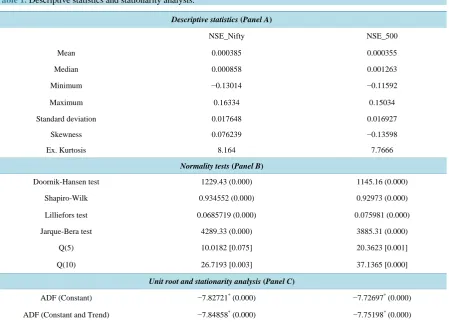
[image:3.595.91.541.383.706.2]

The data set used in this study comprises daily observations of NSE_Nifty and NSE_500 of India over the pe-riod 2006-06-29 to 2012-09-13, a total of 1545 observations. The daily stock returns are defined as the logarith-mic first-difference of the daily closing index values. The data is extracted from the official website of reserve bank of India. We begin with descriptive statistics and stationarity analysis and presented first results in Table 1.

Table 1 of Panel A provides a summary of statistics of the stock return series. The significance of all the

normality tests applied (in Panel B) indicated that the residuals appear to be leptokurtic. Further, the significant Ljung-Box statistics for the returns, Q(5) and squared returns, Q(10), indicating the rejection of the null of white noise, asserting that these return series are auto-correlated. In summary, it is clear that the Indian stock market exhibits frequent volatilities with extensive amplitude (which is also apparent in Figure 1), implying the as-sumption of normal distribution may not be suitable for capturing asymmetry and tail-fatness in a return distri-bution. Finally, unit root and stationary results reported in Panel C of Table 1 indicate that return series is sta-tionary.

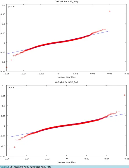
2.4. The Quantile-Quantile Test (Q-Q Plot)

The Q-Q plot helps us to compare shapes of probability distributions by plotting their quantiles against each other.

Table 1. Descriptive statistics and stationarity analysis.

Descriptive statistics (Panel A)

NSE_Nifty NSE_500

Mean 0.000385 0.000355

Median 0.000858 0.001263

Minimum −0.13014 −0.11592

Maximum 0.16334 0.15034

Standard deviation 0.017648 0.016927

Skewness 0.076239 −0.13598

Ex. Kurtosis 8.164 7.7666

Normality tests (Panel B)

Doornik-Hansen test 1229.43 (0.000) 1145.16 (0.000)

Shapiro-Wilk 0.934552 (0.000) 0.92973 (0.000)

Lilliefors test 0.0685719 (0.000) 0.075981 (0.000)

Jarque-Bera test 4289.33 (0.000) 3885.31 (0.000)

Q(5) 10.0182 [0.075] 20.3623 [0.001]

Q(10) 26.7193 [0.003] 37.1365 [0.000]

Unit root and stationarity analysis (Panel C)

ADF (Constant) −7.82721* _{(0.000) −7.72697}* _(0.000)

ADF (Constant and Trend) −7.84858* _{(0.000) −7.75198}* _(0.000)

[image:4.595.89.541.81.657.2]

Figure 1. Exhibiting frequent volatilities for NSE_Nifty and NSE_500.

When we compare two distributions, if the points in the Q-Q plot lies approximately on the line y = x, then both distribution have similar pattern. If the Q-Q plot lies exactly on a line, then the distributions are linearly related. The Quantile-Quantile plots results (Figure 2) suggest that both share common and similar distributions.

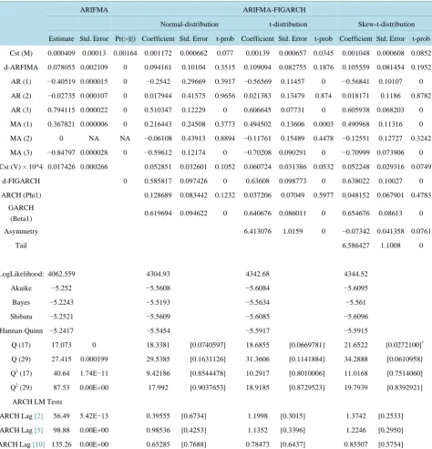
The results obtained from the ARFIMA model (Figure 3), ARFIMA-FIGARCH model and ARFIMA-

-0.15 -0.1 -0.05 0 0.05 0.1 0.15 0.2

2007 2008 2009 2010 2011 2012

NSE_Nifty

-0.15 -0.1 -0.05 0 0.05 0.1 0.15 0.2

2007 2008 2009 2010 2011 2012

[image:5.595.90.532.86.661.2]

Figure 2. Q-Q plot for NSE_Nifty and NSE_500.

FIAPARCH are reported in Table 2 while those are based on Student t-distribution. The ARFIMA model is se-lected using the Akaike Information Criteria (AIC) [16] while fixing AR and MA at the maximum of 3. An ARFIMA (3, d, 3) model is found to best represent the long memory process in stock return series. The esti-mates of d are statistically significant at less than 1% percent level of significance. Thus, the results support that the

-0.15 -0.1 -0.05 0 0.05 0.1 0.15 0.2

-0.06 -0.04 -0.02 0 0.02 0.04 0.06 0.08

Normal quantiles Q-Q plot for NSE_Nifty

y = x

-0.15 -0.1 -0.05 0 0.05 0.1 0.15 0.2

-0.06 -0.04 -0.02 0 0.02 0.04 0.06

Normal quantiles Q-Q plot for NSE_500

[image:6.595.84.538.86.646.2]

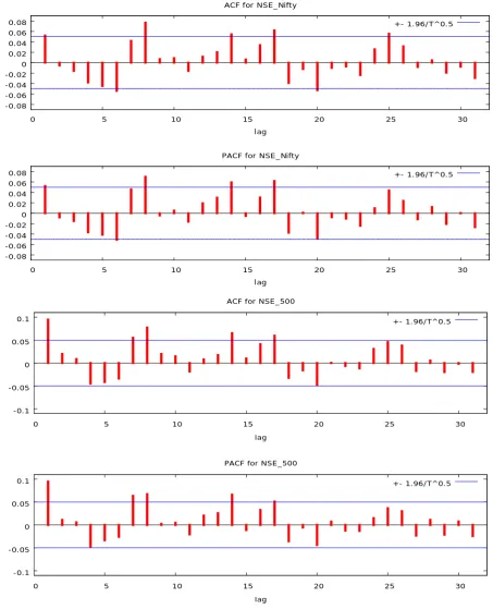
Figure 3. Autocorrelation and partial autocorrelation function for NSE_Nifty and NSE_500.

returns are forecastable and supportive of long memory processes. However, the residuals are mostly negatively skewed, implying that the distribution is non-symmetric. Further, we find significant Q-statistics implying that the residuals are not independent, the J-B test statistics provide the signal that the residuals are leptokurtic and the significant ARCH statistics indicates that the ARCH effects is present in the standardized residuals. There-

-0.08 -0.06 -0.04 -0.02 0 0.02 0.04 0.06 0.08

0 5 10 15 20 25 30

lag ACF for NSE_Nifty

+- 1.96/T^0.5

-0.08 -0.06 -0.04 -0.02 0 0.02 0.04 0.06 0.08

0 5 10 15 20 25 30

lag PACF for NSE_Nifty

+- 1.96/T^0.5

-0.1 -0.05 0 0.05 0.1

0 5 10 15 20 25 30

lag ACF for NSE_500

+- 1.96/T^0.5

-0.1 -0.05 0 0.05 0.1

0 5 10 15 20 25 30

lag PACF for NSE_500

[image:7.595.60.535.100.593.2]

Table 2. Estimation results of the ARFIMA models for NSE_Nifty.

ARIFMA ARIFMA-FIGARCH

Normal-distribution t-distribution Skew-t-distribution

Estimate Std. Error Pr(>|t|) Coefficient Std. Error t-prob Coefficient Std. Error t-prob Coefficient Std. Error t-prob

Cst (M) 0.000409 0.00013 0.00164 0.001172 0.000662 0.077 0.00139 0.000657 0.0345 0.001048 0.000608 0.0852

d-ARFIMA 0.078055 0.002109 0 0.094161 0.10104 0.3515 0.109094 0.082755 0.1876 0.105559 0.081454 0.1952

AR (1) −0.40519 0.000015 0 −0.2542 0.29669 0.3917 −0.56569 0.11457 0 −0.56841 0.10107 0

AR (2) −0.02735 0.000107 0 0.017944 0.41575 0.9656 0.021383 0.13479 0.874 0.018171 0.1186 0.8782

AR (3) 0.794115 0.000022 0 0.510347 0.12229 0 0.606645 0.07731 0 0.605938 0.068203 0

MA (1) 0.367821 0.000006 0 0.216443 0.24508 0.3773 0.494502 0.13606 0.0003 0.490968 0.11316 0

MA (2) 0 NA NA −0.06108 0.43913 0.8894 −0.11761 0.15489 0.4478 −0.12551 0.12727 0.3242

MA (3) −0.84797 0.000028 0 −0.59612 0.12174 0 −0.70208 0.090291 0 −0.70999 0.073906 0

Cst (V) × 10^4 0.017426 0.000266 0.052851 0.032601 0.1052 0.060724 0.031386 0.0532 0.052248 0.029316 0.0749

d-FIGARCH 0 0.585817 0.097426 0 0.63608 0.098773 0 0.638022 0.10027 0

ARCH (Phi1) 0.128689 0.083442 0.1232 0.037206 0.07049 0.5977 0.048152 0.067901 0.4783

GARCH

(Beta1) 0.619694 0.094622 0 0.640676 0.086011 0 0.654676 0.08613 0

Asymmetry 6.413076 1.0159 0 −0.07342 0.041358 0.0761

Tail 6.586427 1.1008 0

LogLikelihood: 4062.559 4304.93 4342.68 4344.52

Akaike −5.252 −5.5608 −5.6084 −5.6095

Bayes −5.2243 −5.5193 −5.5634 −5.561

Shibata −5.2521 −5.5609 −5.6085 −5.6096

Hannan-Quinn −5.2417 −5.5454 −5.5917 −5.5915

Q (17) 17.073 0 18.3381 [0.0740597] 18.6855 [0.0669781] 21.6522 [0.0272100]*

Q (29) 27.415 0.000199 29.5385 [0.1631126] 31.3606 [0.1141884] 34.2888 [0.0610958]

Q2 (17) 40.64 1.74E−11 9.42186 [0.8544478] 10.2917 [0.8010006] 11.0168 [0.7514060]

Q2 _{(29) 87.53 0.00E+00 17.992 [0.9037653] 18.9185 [0.8729523] 19.7939 [0.8392921]}

ARCH LM Tests

ARCH Lag [2] 56.49 5.42E−13 0.39555 [0.6734] 1.1998 [0.3015] 1.3742 [0.2533] ARCH Lag [5] 98.88 0.00E+00 0.98536 [0.4253] 1.1352 [0.3396] 1.2246 [0.2950] ARCH Lag [10] 135.26 0.00E+00 0.65285 [0.7688] 0.78473 [0.6437] 0.85507 [0.5754]

Notes: standard errors and p-values are in parentheses and brackets respectively. ** and * indicate significant at 5 and 1 percent significance level respectively. ln(L) value is the maximized value of the log likelihood function, and AIC is the Akaike (1974) Information criteria. J-B refers to Jarque-Bera normality test. The ARCH(5) and ARCH(10) denotes the ARCH test statistic with lag 5 and 10, while the Q(p) is the Ljung-Box test statistic for standardized residuals at lag p.

[image:8.595.60.538.99.601.2]

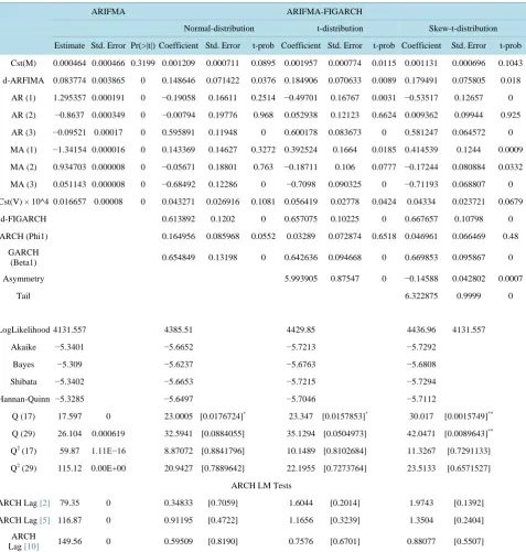
Table 3. Estimation results of the ARFIMA models for NSE_500.

ARIFMA ARIFMA-FIGARCH

Normal-distribution t-distribution Skew-t-distribution

Estimate Std. Error Pr(>|t|) Coefficient Std. Error t-prob Coefficient Std. Error t-prob Coefficient Std. Error t-prob

Cst(M) 0.000464 0.000466 0.3199 0.001209 0.000711 0.0895 0.001957 0.000774 0.0115 0.001131 0.000696 0.1043

d-ARFIMA 0.083774 0.003865 0 0.148646 0.071422 0.0376 0.184906 0.070633 0.0089 0.179491 0.075805 0.018

AR (1) 1.295357 0.000191 0 −0.19058 0.16611 0.2514 −0.49701 0.16767 0.0031 −0.53517 0.12657 0

AR (2) −0.8637 0.000349 0 −0.00794 0.19776 0.968 0.052938 0.12123 0.6624 0.009362 0.09944 0.925

AR (3) −0.09521 0.00017 0 0.595891 0.11948 0 0.600178 0.083673 0 0.581247 0.064572 0

MA (1) −1.34154 0.000016 0 0.143369 0.14627 0.3272 0.392524 0.1664 0.0185 0.414539 0.1244 0.0009

MA (2) 0.934703 0.000008 0 −0.05671 0.18801 0.763 −0.18711 0.106 0.0777 −0.17244 0.080884 0.0332

MA (3) 0.051143 0.000008 0 −0.68492 0.12286 0 −0.7098 0.090325 0 −0.71193 0.068807 0

Cst(V) × 10^4 0.016657 0.00008 0 0.043271 0.026916 0.1081 0.056419 0.02778 0.0424 0.04334 0.023721 0.0679

d-FIGARCH 0.613892 0.1202 0 0.657075 0.10225 0 0.667657 0.10798 0

ARCH (Phi1) 0.164956 0.085968 0.0552 0.03289 0.072874 0.6518 0.046961 0.066469 0.48

GARCH

(Beta1) 0.654849 0.13198 0 0.642636 0.094668 0 0.669853 0.095867 0

Asymmetry 5.993905 0.87547 0 −0.14588 0.042802 0.0007

Tail 6.322875 0.9999 0

LogLikelihood 4131.557 4385.51 4429.85 4436.96 4131.557

Akaike −5.3401 −5.6652 −5.7213 −5.7292

Bayes −5.309 −5.6237 −5.6763 −5.6808

Shibata −5.3402 −5.6653 −5.7215 −5.7294

Hannan-Quinn −5.3285 −5.6497 −5.7046 −5.7112

Q (17) 17.597 0 23.0005 [0.0176724]* _{23.347 [0.0157853]}* _{30.017 [0.0015749]}**

Q (29) 26.104 0.000619 32.5941 [0.0884055] 35.1294 [0.0504973] 42.0471 [0.0089643]**

Q2 _{(17) 59.87 1.11E−16 8.87072 [0.8841796] 10.1489 [0.8102684] 11.3267 [0.7291133]}

Q2 _{(29) 115.12 0.00E+00 20.9427 [0.7889642] 22.1955 [0.7273764] 23.5133 [0.6571527]}

ARCH LM Tests

ARCH Lag [2] 79.35 0 0.34833 [0.7059] 1.6044 [0.2014] 1.9743 [0.1392] ARCH Lag [5] 116.87 0 0.91195 [0.4722] 1.1656 [0.3239] 1.3504 [0.2404]

ARCH

Lag [10] 149.56 0 0.59509 [0.8190] 0.7576 [0.6701] 0.88077 [0.5507]

Notes: Standard errors and p-values are in parentheses and brackets respectively. ** _and * _{indicate significant at 5 and 1 percent significance level respectively.}

Ln(L) value is the maximized value of the log likelihood function, and AIC is the Akaike (1974) Information criteria. J-B refers to Jarque-Bera normality test. The ARCH(5) and ARCH(10) denotes the ARCH test statistic with lag 5 and 10, while the Q(p) is the Ljung-Box test statistic for standardized residuals at lag p.

volatility values are unpredictable. Further, the estimates of fat-tailed parameter (Student (DF)) is also statisti-cally significant at the 1 percent level with the value of is 6.455669, suggesting the usefulness of Student-t dis-tribution in modelling the leptokurtosis of estimated residuals.

is statistically significant at the 1 percent level with value of 7.09, suggesting the usefulness of Student-t distri-bution in modelling the leptokurtosis of estimated residuals. The insignificant diagnostic statistics, for instance, the Q (p), and ARCH (p) also further confirm the selection of Student-t distribution to capture time-varying vo-latility.

In fact, Awartani and Corradi (2005) [17], Tan and Khan (2010) also found that GARCH-class of models that do not allow for asymmetries in the volatility process are beaten by asymmetric GARCH models. As seen in the tables, according to the AIC, the ARFIMA-FIAPARCH models fit the return series better than the ARFIMA- FIGARCH models.

3. Conclusions

It can be concluded that there does exist a non-normal distribution in the return on Indian stock exchange, slightly leptokurtic as indicated by the Jarque-Berra test.

The process is said to be long memory at the long run as long as d > 0 in Equation (1). In particular, for d ∈ (0, 0.5), and d ≠ 0, the series is covariance stationary and mean reverting, with shocks disappearing in the long run; for d ∈ (0.5, 1), the series imply mean-reversion; however, it is not a covariance stationary process as there is no long-run impact of an innovation on future values of the process. For d ≥ 1, the series is non-stationary and non- mean-reversion. On the contrary, the process is said to exhibit intermediate memory, for d ∈ (−0.5, 0). Since our study exhibits that a d value of 0.09, 0.09 and 0.1 is indicative of mean reversion in conflict with efficient mar-ket.

References

[1] Fama, E. (1970) Efficient Capital Markets: A Review of Theory and Empirical Work. Journal of Finance, 25, 383-417. http://dx.doi.org/10.2307/2325486

[2] Bilel, T.M. and Nadhem, S. (2009) Long Memory in Stock Returns: Evidence of G7 Stocks Markets. Research Journal of International Studies, 9, 36-46.

[3] Corhay, A., Rad, A.T. and Urbain, J.P. (1995) Long Run Behavior of Pacific Basin Stock Prices. Applied Financial Economics, 5, 11-18. http://dx.doi.org/10.1080/758527666

[4] Gurgul, H. and Wójtowicz, T. (2006) Long Memory on the German Stock Exchange. Czech Journal of Economics and Finance, 56, 447-468.

[5] Kang, S.H., Cheong, C.C. and Yoon, S.M. (2010) Long Memory Volatility in Chinese Stock Markets. Physica A, 389, 1425-1433. http://dx.doi.org/10.1016/j.physa.2009.12.004

[6] Tan, S. and Khan, M. (2010) Long-Memory Features in Return and Volatility of the Malaysian Stock. Economics Bul-letin, 30, 3267-3281.

[7] Kang, S.H. and Yoon, S.M. (2007) Long Memory Properties in Return and Volatility: Evidence from the Korean Stock Market. Physica A, 385, 597-600. http://dx.doi.org/10.1016/j.physa.2007.07.051

[8] Kang, S.H. and Yoon, S.M. (2008) \Long Memory Features in the High Frequency Data of the Korean Stock Market. Physica A, 387, 5189-5196. http://dx.doi.org/10.1016/j.physa.2008.05.050

[9] Lo, A.W. (1991) Long Term Memory in Stock Market Prices. Econometrica, 59, 1279-1313. http://dx.doi.org/10.2307/2938368

[10] Joyeux, R. and Granger, C.W.J. (1980) An Introduction to Long-Memory Time Series Models and Fractional Differ-encing. Journal of Time-Series Analysis, 1, 15-29. http://dx.doi.org/10.1111/j.1467-9892.1980.tb00297.x

[11] Hosking, J.R.M. (1981) Fractional Differencing. Biometrika, 68, 165-176. http://dx.doi.org/10.1093/biomet/68.1.165

[12] Bailliea, R.T., Bollerslev, T. and Mikkelsenc, H.O. (1996) Fractionally Integrated Generalized Autoregressive Condi-tional Heteroskedasticity. Journal of Econometrics, 74, 3-30. http://dx.doi.org/10.1016/S0304-4076(95)01749-6 [13] Tang T.L. and Shieh, S.J. (2006) Long Memory in Stock Index Future Markets: A Value-at-Risk Approach. Physica A:

Statistical Mechanics and its Applications, 366, 437-448. http://dx.doi.org/10.1016/j.physa.2005.10.017

[14] Cheong, W.C. (2008) Volatility in Malaysian Stock Market: An Empirical Study Using Fractionally Integrated Ap-proach. American Journal of Applied Sciences, 5, 683-688. http://dx.doi.org/10.3844/ajassp.2008.683.688

[16] Akaike, H. (1974) A New Look at the Statistical Model Identification. IEEE Transactions on Automatic Control, 19, 716-723. http://dx.doi.org/10.1109/TAC.1974.1100705

[17] Awartani, B. and Corradi, V. (2005) Predicting the Volatility of S&P-500 Stock Index via GARCH Models: The Role of Asymmetries. International Journal of Forecasting, 21, 167-183.