Investigation of the Scheduler for Heterogeneous Distributed Computing Systems based on Minimal Cover Method

(1)

Investigation of the Scheduler for Heterogeneous

Distributed Computing Systems based on Minimal Cover

Method

S.V.Listrovoy

Ukrainian State Academy of

Railway Transport, 61050,

Kharkov, Ukraine

S.V.Minukhin

Kharkiv National University of

Economics, 61166, Kharkov, Ukraine

S.V.Znakhur

Kharkiv National University of

Economics, 61166, Kharkov, Ukraine

ABSTRACT

The article describes the scheduling system for heterogeneous distributed computing systems. The scheduler based on minimal cover method. The analysis of the effectiveness of the scheduling system for tasks with varying intensity, the law of distribution complexity. The advantage of the method of minimal cover compared to FCFS. A system of rules for the optimization of the proposed planning changes in the intensity and complexity of tasks.

General Terms

The procedure for scheduling tasks for clusters

Keywords

Grid system, task scheduling, scheduling algorithm, minimal cover, statistical analysis, intensity, complexity

1. INTRODUCTION

Exploitation of modern Grid systems is related to the necessity of improvement of their performance. It is defined by such metrics as utilization resources, run time of all tasks on the resources, total time completion of the tasks set later than other ones, etc.

Now large amount of papers is devoted to the comparative analysis batch scheduling methods [1–14]. For example, a detailed description and classification scheduling algorithms for Grid computing is given in [12, 13, 14].

We investigated articles that examine the most common method of FCFS, the main advantage of which is the lack of information on the requirements of task (a method scheduling the task, standing first in order in query for the first free resource), with batch modes [6–9]. However, FCFS has significant disadvantages: its efficiency decreases sharply with increasing intensity of tasks flows and the heterogeneity of computing environment: resource queues are formed, which greatly degraded the utilization of resources due to their inactivity [8, 9]. More preferred is batch scheduling mode. In this mode the important point is the timing (mapping events) and frequency scheduling, largely impact on the performance metrics – minimize makespan and the total execution time of all tasks [10, 11].

Since there is a tendency for increase of the number of heterogeneous computing clusters and of the tasks with differentiated solutions complexity (execution time), it is relevant to use more fine-tuning of scheduling process (procedure), which will allow to "pack" set of resources effectively on the one hand, and to provide a high load of all resources on the other hand. This can be achieved through the use of scheduling algorithms and additional components (modules) in the mechanism of Grid resources scheduling.

2. GRID SCHEDULING MODEL

Grid systems schedulers are main components in an interconnected information-communication system of Grid. Grid uses various concepts of schedulers based on online and offline modes. An immediate mode scheduler only considers a single task for scheduling on a FCFS (first come first served) basis while a batch mode scheduler considers a number of tasks at once for scheduling. Scheduling onto the Grid is NP complete [1]. Therefore, the problem of choosing an effective method of scheduling is difficult. As a rule the performance of various scheduling algorithms in the frames of common Grid scheduling mechanism, should be compared. When comparing the results of the various scheduling systems operation, evaluations of scheduler’s efficiency are not always correct and comparable. This is due to the complexity of the analysis of the timing characteristics of the tasks solution in various systems and load of resources to run incoming tasks.

The purpose of this paper is development of a new scheduling method, which is based on a model problem of the minimal cover. Two main ideas are the basis for the proposed approach: at each step to schedule the batch of tasks and at each step for their running to allocate the minimum number of free and available resources.

Feature of this method is that it uses the statistical characteristics that define the Grid environment.

So main objectives of this study are:

analysis of statistical laws identified in the process of using the proposed tasks scheduling mechanism for heterogeneous Grid system during the change of characteristics of the flow of incoming tasks (workflows); justification of selection of optimal parameters values of mechanism components for improvement of its efficiency;

to develop a system of rules based on the results of statistical analysis of the Grid system exploitation, which allows to determine the optimal values of parameters of scheduling mechanism components for all characteristics of tasks and resources, and thus to improve the performance of Grid system.

The goal of the proposed method is to minimize the total execution time, has to be chosen in order to utilize the performance resources to minimize execution time on all resources and maximized average resource utilization.

(2)

about available resources. Availability of adequate resources for the given task depends not only on the condition of resources, but also on the policy of their use followed by resource managers or by administrators of a virtual organization. Currently, various strategies are used for resources allocation to distribute tasks between resources (e.g. push-model or pull-model). It is suggested to use strategy in the proposed scheduling mechanism: batch of task is scheduling on the available resources, however, the tasks may be in the scheduler until some resource becomes available, and then the most appropriate task selected for the allocated resource. We consider following assumptions about task:

all tasks are independent;

tasks are non-preemptive: their execution on a resource cannot be suspended until completion;

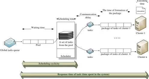
all resources have the different computing capability. It should be noted that the services performing tasks monitoring, tasks restart and resources monitoring are implemented within the Grid system itself and are not components of scheduling mechanism. According to scheme in Fig. 1, the tasks from the global tasks queue come to pool with a certain frequency and intensity. Pool is a stack for temporary storage of incoming tasks. The pool size is determined by the maximum intensity of incoming tasks: if the pool size is less than the number of incoming tasks, an additional queue will be created already at the entrance of the system itself. Tasks are unloaded at regular intervals which defined by scheduling cyclicity, from the pool to the block of scheduling, where the scheduling algorithm is implemented. To minimize the time of scheduling a fast approximate algorithm for solving the problem

of the minimal cover is used [17, 18]. Scheduling time (working time of algorithm for solving the problem of the minimal cover) depends on the size of the pool, i.e. the number of the tasks coming on the scheduling block, and the number of available recourses and free ones at the time of scheduling. The approximate scheduling algorithm provides a solution to the task in polynomial time O(mn2)[18]), so the cyclicity of approximate should be more than time for solving the scheduling task. As a result of scheduling tasks are assigned to free elements of the blocks of tasks package (package must have at least one free element) of correspondent resources, i.e. those which are not filled completely at the time of scheduling (see Fig. 1).

It should be noted that tasks are coming with a delay, which determines the communication delay and data transfer from the scheduling block to resources for their execution.

The presence of a package of tasks in this mechanism is due to the need to solve two problems:

1) creating artificial queues for each resource that helps to prevent possible downtime and increases the coefficient of utilization of resources;

2) creation of managed package of tasks for the possibility of scheduling and assignment of tasks on the level of the resource itself (if the resource is a cluster or a multiprocessor system).

This study is used a serial mode for performing tasks on each resource, i.e., the tasks to be performed on the resource are sequentially selected from the tasks package as a resource becomes de-allocated (free).

package of tasks of cluster 1

Cluster n Cluster 1

package of tasks of cluster n

tasks

Scheduler _tasks

….

Pool

A set of tasks from the pool

Global tasks queue

Scheduling cyclicity

Response time of task (time spent in the system)

Schedulingtime

Waiting time

Communication delay

The time of formation of the package

execution Executing

[image:2.595.56.552.386.647.2]

time

Fig 1: The overall architecture of ascheduling mechanism

The mathematical formulation of the scheduling model is a problem linear Boolean programming [12]:

₍ ₎ _min

1







 k

n

j j

t x t

L

, (1)

with, subject to the constraints

 

0,1, ) ( }; 1 , 0 {

; , 1 i , 1 1

) (

 

  



k ij

t j x

m n

j

t j x 

(3)

where m is a number of tasks, which should be scheduled; n is a number of the resources that are available and not allocated (free) at the time of scheduling; tk



[T0, TN].

Scheduling is carried out on the time interval [T0, TN], where T0

is the time of scheduling start; TN is the completion time for

scheduling all tasks from global queue.

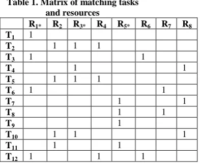
The problem (1), (2) can be regarded as a minimal cover (MC) problem – determining the minimum number of columns in the Boolean matrix B, which covers all rows of the given matrix whose elements in the context of solving the scheduling problem are interpreted as follows: columns correspond to the non-allocated at the time of scheduling grid system resources, rows correspond to the tasks, subject to scheduling, which must be resolved on these resources (Table 1).

This approach is based on the following assumptions. 1. The scheduling system is organized in a two-level structure. A set of tasks (pool) which should be scheduled to which the method of solving the MC problem (1), (2) should be applied, is formed on the first level. Next, the tasks selected as a result of its solving scheduled to the available and free at the time of scheduling resources, and will be solved there under the control of the local scheduler.

2. The scheduling method at each step of scheduling maximally loads the minimum number of resources which are free and available at the time of scheduling. Thus, for subsequent distribution of the task in a queue, the amount of resources available for possible tasks allocation will be maximal.

3. Method (algorithm) for task scheduling (1), (2) must have a low complexity of its realization in order to minimize the time spent for tasks scheduling for their execution on free resources. 4. The scheduling system utilizes package technology «pull-push» so that firstly the tasks, organized as a batch of tasks (pool), become taken from the global queue (pull). When they will be scheduled on resources, they will be placed into a task package on the allocated resource (resources) and then transferred for a execution (push) onto this resource (resources). 5. At scheduling time points tkm tasks are independent and n

[image:3.595.54.251.480.641.2]

resources for allocation are available and free.

Table 1. Matrix of matching tasks and resources

R1* R2 R3* R4 R5* R6 R7 R8 T1 1

T2 1 1 1

T3 1 1

T4 1 1

T5 1 1 1

T6 1 1

T7 1 1

T8 1 1

T9 1

T10 1 1 1

T11 1 1

T12 1 1 1

The following metrics are usually used as performance metrics (objectives) of the scheduler in Grid system: the execution time of all tasks in a global queue and resources utilization.

Mean time of one task processing is determined by the formula:

ion_time sk_complet average_ta

T ₌



 N

i i

t

N

1

, execution

1

(3)

where N is the number of tasks in the global queue.

Execution time of all tasks in a queue TN computed as follows:

T_N T_lastT_first, (4)

where

T

_first is the arrival time of the first task in the queue;

last

T

is the time of completion of the last task in a queue.

The coefficient of the utilization K_util of resource Rj is given by:

, N T

R T util

K  i ₍₅₎

where TRi is the execution (completion) time for all tasks in the global queue which were scheduled on resource Rj.

3. STATISTICAL

ANALYSIS

OF

SIMULATION

RESULTS

AND

FORMALIZATION

OF

RULES

OF

SCHEDULING

To carry out computing experiments a simulation model of the Grid scheduling system is used, based on the use of MC algorithm [18] with the complexity O (mn2). Internal time of simulation model (one cycle) is used as a time unit of scheduling and computing in the program. This internal time corresponds to the time for one task execution which has the complexity of 1000 MI on the resource characterized by 1000 MIPS performance.

Computing experiment involves the study of scheduling for two types of tasks:

 tasks having low computational complexity, which have a mean complexity value up to 500 cycles (which corresponds to the time of the task completion of less than 100 ms);

 tasks having high computational complexity, with its mean value of 30,000 cycles (which corresponds to the time of the task completion up to 8 hours).

The following parameters were chosen for imitational simulation.

For the first group of tasks from input flow random normal distribution law was selected. The total number of tasks in the global queue was 2100; the complexity of the task varied in the range from 20 to 320; the intensity of the tasks varied in the range from 5 to 40 task with step 5; the universality of task (the percentage of available resources, which can be used for one task execution – analogue of the heterogeneity of resources) was 50%; the length of the pool was 100 (the maximum number of tasks filled (downloaded) in the pool at the same time, or as they come into the system for execution); scheduling cyclicity varied from 1 to 40 cycles; a task packages to resources was chosen 5; amount of resources was 10; single resource productivity (performance) was 5 cycles; communication delay was 1 cycle.

For the second group of tasks from input flow random normal distribution law was selected. The total number of tasks in the global queue was 1000; the complexity of one task was 30000; complexity variance was 1000 cycles; the intensity of the tasks varied in the range from 50 to 250 with step 50; the universality of tasks was 50%; the length of the pool was 100; scheduling cyclicity varied in the range from 1 to 5 cycles; the task package size was 10; amount of resources varied from 5 to 30, single resource productivity (performance) was 10 cycles, the communication delay was 20 cycles.

(4)

only by comparing them with the number of available resources. If there are more resources than tasks, intensity is low, otherwise it is high.

These statistical results of simulation are mean values of measures obtained on the basis of 20 tests (samples) generated. To ensure the adequacy of the experiments conducted, total tasks complexity and their number for the generated samples is the same for each test.

The experimental results showed that the greatest influence on scheduling mechanism (procedure) is made by the intensity of the input tasks flow and their computational complexity, and that the main control parameters for the effective scheduling procedure are the pool size and scheduling cyclicity.

The main task of the scheduler is the optimal «packing» tasks on resources, therefore input intensity of the tasks will be transformed by scheduler during each scheduling cycle into tasks packages to N resources. The maximum intensity of the tasks incoming on the resources during each scheduling cycle can be computed using the following equation:

).

_

/(

)

_

(

pool

size

number

of

resourses

(6)

The higher scheduling cyclicity (greater periodicity), the greater the number of tasks enters the pool and then assigned to the tasks packages during each scheduling cycle. In the case of high task input intensity or high scheduling cyclicity pool will be fully loaded and, thus, determines the maximum number of tasks involved in the scheduling procedure.

For tasks with low intensity and low computational complexity, optimal organization of the scheduling procedure assumes that the tasks packages for each resource should include only one task. This ensures minimal task downtime in the system and uniform resources load due to the fact that any time at least one task from the package will always enter the resource which is free at this particular moment of time.

If the flow of tasks with high intensity or high computational complexity is present, the scheduling is carried out for future, i.e. tasks are in queue in the pool or in a task package. The increase of scheduling periodicity (cyclicity decrease) allows to increase the number of task in task package for each resource; the increase of scheduling cyclicity allows to increase the time of task presence in the pool. Accordingly, with decreasing of scheduling cyclicity it is necessary to increase the

tasks package size up to a maximum (according to equation (6)), otherwise the pool size should be increased to a value of maximum intensity of the input task flow.

Results of statistical analysis of scheduling procedure for tasks with small computational complexity depending on the change of their flow intensity and scheduling cyclicity are shown in Fig. 2, 3. The Figures showing that for given task type an execution time is linearly dependent on scheduling cyclicity, i.e. execution time increases with increasing cyclicity. Studies are showing that if other characteristics being equal, minimum scheduling cyclicity, which is equal to one cycle, yields the smallest value of execution time. This relationship holds when task complexity is greater than 1 cycle.

When the intensity of tasks flow is increasing the linear dependence remains unchanged, but the gain from scheduling cyclicity change decreases. With increasing of intensity to a value more than 100 task, change of scheduling cyclicity does not affect the time of tasks completion. This is due to the fact that the pool limits the number of task entering for the task scheduling.

To obtain positive effect by changing scheduling cyclicity it was suggested to use the equation (7), which allows to define the upper bound of scheduling cyclicity. It should be noted that when the input intensity of tasks increases, the average number of tasks in the pool will also increase. This leads to the possibility to increase the scheduling cyclicity without sacrificing overall tasks completion time for fixed values of other characteristics.

Unlike the overall tasks completion time, the mean response time (the mean completion time of one task) shows a nonlinear relationship. In cases when scheduling cyclicity is less than the mean time for a resource deallocation (in this case it is 5 cycles, which is less than the ratio (30 cycles is task complexity) / (5 cycles of the resource productivity)), the queue of the incoming scheduled tasks will be formed in the system. These tasks await release of the resource, which leads to a sharp increase in response time.

With increasing of scheduling cyclicity tasks waiting time in the queue decreases because during this time most of the previous tasks from the pool will be completed already. For large cyclicity values response time of task includes only time spent in the pool + transportation time (communication delay time) + task completion time on the resource (Fig. 1), which determines it’s the minimum value.

). resources of

e performanc average

tasks of y versatilit complexity

average (

/ ) tasks of complexity average

pool in the tasks of number average (

 

(5)

Scheduling cyclicity, cycle

E

xe

cu

ti

o

n

t

ime

,

cyc

le

intensity of tasks : 5 intensity of tasks : 10 intensity of tasks : 15 intensity of tasks : 20 intensity of tasks : 40

-5 0 5 10 15 20 25 30 35

-10000 0 10000 20000 30000 40000 50000 60000

Fig 2: The dependence of tasks execution (completion) time on the scheduling cyclicity and intensity of tasks

The maximum value of the coefficient of resources use is possible in the case of a constant resources load (their idle time minimization). This could be achieved by an intensity increase, or by decrease of scheduling cyclicity. Thus, at low intensity of 5 (less than the amount of resources), scheduling cyclicity should

be equal to one cycle, at an intensity of 20 scheduling cyclicity must be no more than 5 cycles, at high intensity of 40 scheduling cyclicity, which ensures a high load of resources will be equal to 10 cycles.

U

ti

li

za

ti

o

n

co

e

ff

ici

e

n

t

intensity of tasks : 5 intensity of tasks : 10 intensity of tasks : 15 intensity of tasks : 20 intensity of tasks : 40

-5 0 5 10 15 20 25 30 35

0,0 0,1 0,2 0,3 0,4 0,5 0,6 0,7 0,8 0,9

Fig 3: Dependence of the utilization coefficient on the scheduling cyclicity and intensity of tasks flow

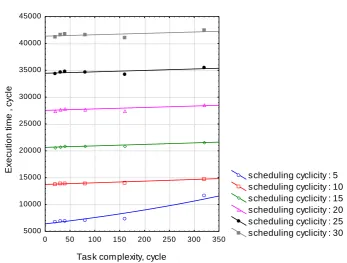
To analyze the effect of changes in task characteristics on scheduling procedure in this study we separately analyzed the effect of the tasks complexity (work content) growth on the results (effectiveness) of scheduling. It should be noted that as the complexity of the task is measured in cycles, the study used a

(6)

almost linearly dependent on the increasing complexity of the task, which is typical for all selected scheduling cyclicities.

However, with increasing task complexity utilization of the resource begins to exponentially depend on scheduling cyclicity, even at low intensity of tasks (Fig. 5). Thus, when the complexity of tasks equal to 160 and 320, there is a maximum loading of resources (utilization coefficient is close to 1), which could be explained by the queue of tasks appearance on resources.

Here we will consider scheduling results in the conditions of changing amount of resources for tasks having large computational complexity. The peculiarity of these tasks is that in a real Grid system they can be completed during the time from several hours to several days. In virtual organizations, the share of such tasks is quite high, and administrators must to explicitly allocate tasks of high complexity in a separate queue, and to prescribe certain rules of scheduling for them.

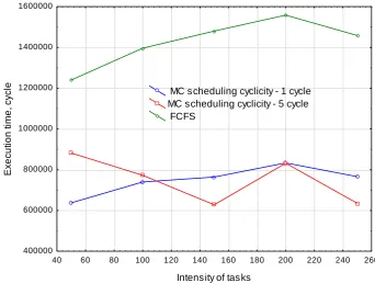
Figs. 6, 7 shows the change in completion time of all tasks in the queue depending on scheduling cyclicity (for the MC algorithm) and comparison of this time with the completion time obtained using the FCFS algorithm. It should be noted that scheduling efficiency of a high complexity tasks is not significantly affected by tasks package size or scheduling periodicity. For example, for only 5 resources run time of tasks with great complexity does not depend on scheduling periodicity and tasks intensity. After a few scheduling cycles task queues will be generated for resources and further scheduling is carried out "for future ". However, it should be noted that the proposed “list algorithm” MC has a considerable advantage in relation to FCFS due to possibility of the optimum packing of resources. In

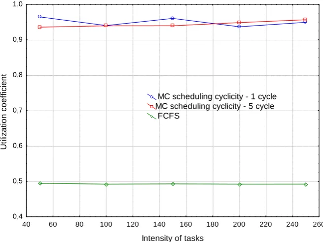
Fig. 6 gain in the tasks run-time is up to 45%. Increasing the number of resources to 30 leads to the effect of reducing of tasks completion time, but intensity increase leads to linear increase of this indicator value, which indicates that resources are underloaded (Fig. 7). A similar result shown in the diagrams in Fig. 8, 9. For a linear change of tasks intensity for 5 resources “list algorithm” MC shows the highest value of utilization coefficient (0.95), suggesting that there is a queue before each resource. Unlike MC, FCFS allows to load only 50% of the resources (0,5). Increasing the number of resources to 30 leads to a decrease of utilization coefficient for MC method making its efficiency to be close to the efficiency of FCFS. Consequently, the gain for tasks having great complexity for MC algorithm can be obtained in the case of a small amount of free resources, or high tasks intensity.

Based on the results of experiments conducted in order to calculate the lower limit of scheduling cyclicity value for known minimal task complexity, the following heuristics have been found which can be described by equation (8). Equation (8) is valid provided that pool size (or intensity) is greater or equal to the amount of resources. In this case scheduling cyclicity is determined to a greater extent by minimal time of resource deallocation i.e. by the ratio (minimal task complexity / maximum resource performance).

Because pool size can be changed and set equal to the amount of resources it is always possible to ensure a minimal completion time of all tasks and maximal resources utilization coefficient in the proposed scheduling mechanism.

Thus, the desired problem can be reduced to the problem of resources scheduling process management.

).

ty

productivi

resource

maximum

*

resources

of

number

(

/

)

complexity

tasks

minimal

*

intensity

tasks

average

(

(8)

Task complexity, cycle

E

xe

cu

ti

o

n

t

ime

,

cyc

le

scheduling cyclicity : 5 scheduling cyclicity : 10 scheduling cyclicity : 15 scheduling cyclicity : 20 scheduling cyclicity : 25 scheduling cyclicity : 30

0 50 100 150 200 250 300 350

5000 10000 15000 20000 25000 30000 35000 40000 45000

[image:6.595.125.473.440.703.2]

(7)

U

til

iz

a

tio

n

c

o

e

ff

ic

ie

n

t

task complexity : 20 task complexity : 30 task complexity : 40 task complexity : 80 task complexity : 160 task complexity : 320

4 6 8 10 12 14 16 18 20 22 24 26 28 30 32 -0,2

0,0 0,2 0,4 0,6 0,8 1,0

Fig 5: Dependence of the utilization coefficient on scheduling cyclicity for the tasks of various complexities

40 60 80 100 120 140 160 180 200 220 240 260

Intensity of tasks

400000 600000 800000 1000000 1200000 1400000 1600000

E

xe

cu

ti

o

n

t

ime

,

cyc

le _{MC scheduling cyclicity - 1 cycle}

[image:7.595.125.468.350.608.2]

MC scheduling cyclicity - 5 cycle FCFS

(8)

40 60 80 100 120 140 160 180 200 220 240 260

Intensity of tasks

180000 190000 200000 210000 220000 230000 240000 250000 260000 270000

E

xe

cu

ti

o

n

t

ime

,

cyc

le

[image:8.595.127.471.72.334.2]

MC scheduling cyclicity - 1 cycle MC scheduling cyclicity - 5 cycle FCFS

Fig 7: Dependence of completion time values for MC and FCFS schedulers for various intensities and tasks scheduling cyclicities with high computational complexity for 30 resources

40 60 80 100 120 140 160 180 200 220 240 260

Intensity of tasks

0,4 0,5 0,6 0,7 0,8 0,9 1,0

U

ti

liza

ti

o

n

co

e

ff

ici

e

n

t

[image:8.595.134.462.388.634.2]

(9)

40 60 80 100 120 140 160 180 200 220 240 260

Intensity of tasks

0,40 0,42 0,44 0,46 0,48 0,50 0,52 0,54 0,56 0,58 0,60 0,62 0,64

U

ti

li

za

ti

o

n

co

e

ff

ici

e

n

t

[image:9.595.126.470.73.336.2]

Fig 9: Dependence of utilization coefficient values for MC and FCFS schedulers for various intensities and tasks scheduling cyclicities with high computational complexity for 30 resources

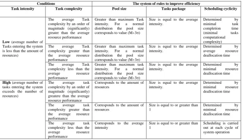
Description of the system of rules for effective scheduling of resources load is shown in Table 2. The system of rules includes recommendations on setting up three main parameters of scheduling mechanism, which should be installed simultaneously

when intensity conditions, distribution law and tasks characteristics will be changing.

Table 2. The rules for setting up scheduling mechanism parameters when task characteristicschange

Conditions The system of rules to improve efficiency

Task intensity Task complexity Pool size Tasks package Scheduling cyclicity

Low (average number of Tasks entering the system is less than the amount of resources)

The average Task complexity by an order of magnitude (significantly) greater than the average resource performance

Greater than maximum Task intensity. For a normal distribution the pool size corresponds to value (M+3σ)

Size is equal to the average intensity.

Determined by

minimal task

completion time (minimal tasks computational complexity) The average Task

complexity greater than the average resource performance

Greater than maximum task intensity. For a normal distribution the pool size corresponds to value (M+3σ)

Determined by

average resource deallocation time

The average Task complexity less than the

average resource

performance

Greater than maximum task intensity. For a normal distribution the pool size corresponds to value (M+3σ)

Determined by

minimal resource deallocation time

High (average number of tasks entering the system exceeds the number of resources)

The average task complexity by an order of magnitude (significantly) greatere than the average resource performance

Corresponds to the amount of resources

Determined by

The average task complexity greater than the average resource performance

Corresponds to the amount of resources

Size is equal to or greater than 1

Determined by

The average task complexity less than the

average resource

performance

Corresponds to the average intensity

Size is equal to or greater than 1

[image:9.595.49.549.456.745.2]

(10)

4. CONCLUSIONS

1. The effectiveness of the proposed scheduling mechanism depends on the interaction of scheduling and pool setting, scheduling block, tasks packages for resources. Our studies have shown that the most important parameter influencing scheduling efficiency is the scheduling cyclicity. Optimally chosen scheduling cyclicity allows to minimized the influence of intensity dynamics and incoming tasks complexity.

2. Selection of the optimal scheduling cyclicity depends on resource deallocation time. Scheduling cyclicity must be less than average resource deallocation time for a given tasks complexity and resource performance.

3. Resources utilization coefficient and all tasks completion time have an inverse relationship. Utilization coefficient increase leads to a linear decrease of all tasks completion time. The empiric dependence (3) found as a result of the conducted experiments allows to calculate the expected tasks completion time in case if the certain level of resources load must be ensured in the system.

4. The results obtained indicate a close relationship of various Grid system efficiency indicators and allow to provide resources scheduling processes management in these systems based on the choice of resources load maximization strategy or strategy for average response time minimization for the task.

Future work will be to continue the study in the direction of the comparative analysis of effectives cover algorithms (for example, greedy algorithms) with the presented in this paper approximation algorithm. The study also involves evaluating the use of the approximation algorithm in Maui for scheduling in heterogeneous distributed systems.

REFERENCES

[1] M. Maheswaran, S. Ali, H. J. Siegel, D. Hensgen, R. F. Freund.

"

Dynamic mapping of a class of independent tasks onto heterogeneous computing systems", Journal of Parallel and Distributed Computing, no. 59(2), pp. 107 – 121, 1999.

[2] F. Xhafa, L.Barolli, A. Durresi.

"

Batch mode scheduling in grid systems

"

, Int. J. Web and Grid Services, no. 3(1), pp. 19 – 37, 2007.

[3] F. Xhafa, A. Abraham.

"

Meta-heuristics for Grid Scheduling Problems

",

Meta. for Sched. in Distri. Comp. Envi., SCI 146, pp. 1–37, 2008.

[4] T. D. Braun, H. J. Siegel, N. Beck, Ladislau L. Boloni, R. F. Freund, D. Hensgen, M. Maheswaran, A. I. Reuther, J. P. Robertson, M. D. Theys, B. Yao. "A comparison of eleven static heuristics for mapping a class of independent tasks onto heterogeneous distributed computing systems", Journal of Parallel and Distributed Computing, no. 61(6): pp. 810 – 837, 2001.

[5] J. Smith, J. Apodaca, Anthony A. Maciejewski, H. J. Siegel.

"

Batch Mode Stochastic-Based Robust Dynamic Resource Allocation in a Heterogeneous Computing System

",

In Proceedings of PDPTA'2010, pp. 263 – 269, 2010.

[6] Ashish Chandak, Bibhudatta Sahoo, Ashok Kumar. Turuk.

"

An Observation on Performance Analysis of Grid Scheduler", IJCST, no. 2 (4), pp. 516–520, 2011.

[7] Bibhudatta Sahoo, Aser Avinash Ekka. Performance

"

Analysis Of Concurrent Tasks Scheduling Schemes In A

Heterogeneous Distributed Computing System

",

In Proceedings of the National Conference on Computer Science and Technology, 11-12 Nov 2006, KIET, Ghaziabad.

[8] Issam Al-Azzoni, Douglas G. Down.

"

Dynamic Scheduling for Heterogeneous Desktop Grids

"

, Journal of Parallel and Distributed Computing, no. 70(12), pp. 1231–1240, 2010.

[9] Jong-Kook Kima, Sameer Shivleb, Howard Jay Siegelb, Anthony A. Maciejewskib, Tracy D. Braunb, Myron Schneiderb, Sonja Tidemanc, Ramakrishna Chittac, Raheleh B. Dilmaghanib, Rohit Joshib, Aditya Kaulb, Ashish Sharmab, Siddhartha Sripadab, Praveen Vangarib, Siva SankarYellampallie.

"

Dynamically mapping tasks with priorities and multiple deadlines in a heterogeneous

environment

",

J. Parallel Distrib. Comput., no. 67, pp. 154 – 169, 2007.

[10]HE Xiaoshan, Xian-He Sun, Gregor von Laszewski.

"

QoS Guided Min-Min Heuristic for Grid Task Scheduling

"

, Journal of Computer Science and Technology - Grid computing, no 18 (4), pp. 442 – 451, 2003.

[11] Abdul Aziz, Hesham El-Rewini.

"

Grid Resource Allocation and Task Scheduling for Resource Intensive Applications

",

http://www.cecs.uci.edu/~papers/icpp06/ICP PW/papers/008_aaziz-grid.pdf.

[12]J. Schopf. "Ten Actions When SuperScheduling, document of Scheduling Working Group", Global Grid Forum, July 2001, http://www.ggf.org/documents/GFD.4.pdf.

[13]H. Chen and M. Maheswaran.

"

Distributed Dynamic Scheduling of Composite Tasks on Grid Computing Systems

"

, In Proc. of the 16th International Parallel and Distributed Processing Symposium (IPDPS 2002), pp. 88– 97, Fort Lauderdale, Florida USA, April 2002.

[14]Fangpeng Dong and Selim G. Akl.

"

Scheduling Algorithms for Grid Computing: State of the Art and Open Problems

",

Technical Report No. 2006-504 School of Computing, Queen's University Kingston, Ontario January 2006.

[15]S. Tuecke, K. Czajkowski, I. Foster, S. Graham, C. Kesselman, P. Vanderbilt and D. Snelling.

"

Grid Service Specification, Open Grid Service Infrastructure Working Group (OGSI)", Global Grid Forum, http://www.cs.ucy.ac.cy/crossgrid/cygriddl/gsspec.pdf.

[16]Job Submission Description Language (JSDL) Specification, http://forge.gridforum.org/projects/jsdl-wg.

[17] S.V. Listrovoy, A.Yu. Gul. "Method of Minimum Covering Problem Solution on the Basis of Rank Approach

",

Engineering Simulation, 1999, Vol. 17, pp. 73–89.

[18] S.V. Listrovoy, S.V. Minukhin.

"

Method for solving the minimum vertex cover in a an arbitrary graph and the