Evaluating Volatility Forecasts in Option
Pricing in the Context of a Simulated
Options Market
Xekalaki, Evdokia and Degiannakis, Stavros
Department of Statistics, Athens University of Economics and
Business
2005
Online at
https://mpra.ub.uni-muenchen.de/80468/
E v a l u a t i n g V o l a t i l i t y F o r e c a s t s i n O p t i o n P r i c i n g i n t h e
C o n t e x t o f a S i m u l a t e d O p t i o n s M a r k e t
Evdokia Xekalaki and Stavros Degiannakis
Department of Statistics, Athens University of Economics and Business
Abstract
The performance of an ARCH model selection algorithm based on the standardized
prediction error criterion (SPEC) is evaluated. The evaluation of the algorithm is performed by comparing different volatility forecasts in option pricing through the simulation of an
options market. Traders employing the SPEC model selection algorithm use the model with the lowest sum of squared standardized one-step-ahead prediction errors for obtaining their
volatility forecast. The cumulative profits of the participants in pricing one-day index straddle options always using variance forecasts obtained by GARCH, EGARCH and TARCH models
are compared to those made by the participants using variance forecasts obtained by models suggested by the SPEC algorithm. The straddles are priced on the Standard and Poor 500 (S & P 500) index. It is concluded that traders, who base their selection of an ARCH model on
the SPEC algorithm, achieve higher profits than those, who use only a single ARCH model. Moreover, the SPEC algorithm is compared with other criteria of model selection that
measure the ability of the ARCH models to forecast the realized intra-day volatility. In this case too, the SPEC algorithm users achieve the highest returns. Thus, the SPEC model
selection method appears to be a useful tool in selecting the appropriate model for estimating future volatility in pricing derivatives.
1 . I n t r o d u c t i o n
ARCH models have widely been used in financial time series analysis and particularly in analyzing the risk of holding an asset, evaluating the price of an option, forecasting time varying confidence intervals and obtaining more efficient estimators under the existence of heteroscedasticity. In the recent literature, numerous parametric specifications of ARCH models have been considered for the description of the characteristics of financial markets. The richness of the family of parametric ARCH models certainly complicates the search for the true model, and leaves quite a bit of arbitrariness in the model selection stage. The problem of selecting the model that describes best the movement of the series under study is therefore of practical importance.
Degiannakis and Xekalaki (1999) made a comparative study of the forecasting ability of ARCH models based on a standardized prediction error criterion (SPEC). According to their SPEC based model selection algorithm, the models with the lowest sum of squared standardized one-step-ahead prediction errors are the most appropriate to exploit future
volatility. In this paper, inspired by Engle et al.’s (1993) approach to assess incremental
profits for a set of competing forecasts of the variance for a given portfolio, we examine the usage of the SPEC model selection algorithm, in pricing contingent claims. The goal of the paper is to evaluate the SPEC algorithm for volatility model selection through the simulation of an options market. In particular, in section 2, the ARCH process is presented. Section 3 provides a description of the SPEC model selection algorithm in the context of ARCH
models, while section 4 presents Engle et al.’s (1993) data generated set-up of evaluating
volatility forecasts. In sections 5 and 6, based on Engle et al.’s (1993) technique, the
suggested model selection method is evaluated using daily return data for the S&P500 stock index over the period from June 26th, 1991 to October 18th, 2002. The use of a model selection method is a tedious procedure as it presupposes the estimation of a set of models. In order to examine whether there is any added value in using the suggested model selection algorithm instead of any other method of using only a single ARCH model in the study, the performance of the SPEC algorithm in investigated against a set of such methods for a range of ARCH models. The results of section 5 provide evidence that this is indeed the case since they indicate that the SPEC model selection algorithm offers a useful tool in providing information related to the appropriate model. In section 6, the algorithm is compared with other methods of model selection. In particular, model selection criteria that measure the accuracy of the models to predict the realized volatility are constructed. The SPEC method is then compared with those model selection methods. Clearly, the SPEC algorithm outperforms all of the other methods of model selection considered. Finally, in section 7 a brief discussion of the results is provided.
2 . T h e A u t o r e g r e s s i v e C o n d i t i o n a l H e t e r o s c e d a s t i c i t y ( A R C H ) P r o c e s s
Let
yt refer to the univariate discrete time real-valued stochastic process to bepredicted (i.e. the rate of return of a particular stock or market portfolio from time
t
1
tot
), where E
yt |It1
Et1
yt
t denotes the conditional mean given the information setavailable at time
t
1
, It1. The innovation process for the conditional mean,
t , is thengiven by
t yt
t with zero unconditional mean, unconditional variance
2
2t
t
E
V
and E
t
s
0,
t
s
. The conditional variance of the process isallowed to depend on It1 and is given by
2 2 11 t t t t
t
y
E
V
. Since investors would know the information set It1 when they make their investment decisions at timet
1
, therelevant expected return to the investors and volatility are
t and2
t
An ARCH process,
t , can be presented as:t t t z
,where
0, 1
~
. . .
t
t d
i i
t f E z V z
z ,
and
1,
2,...;
1,
2,...;
1,
2,...
2
t t t t t tt
g
,(1)
where
zt is a sequence of independently and identically distributed random variables,
.
f
is the density function of zt,
t is a time-varying, positive and measurable function ofthe information set at time
t
1
,
t is a vector of predetermined variables included in It and
.
g
could be a linear or nonlinear functional form that has been considered in the ARCH literature. By definition,
t is serially uncorrelated with mean zero, but with a time varyingconditional variance equal to
t2. The conditional variance is a linear or nonlinear function oflagged values of
t and
t and predetermined variables included in It1,
t1,
t2,...
. Thestandard ARCH models assume that
f
.
is the density function of the normal distribution. However, Bollerslev (1987) proposed using the student t distribution with an estimated kurtosis regulated by the degrees of freedom parameter. Nelson (1991) proposed using the generalized error distribution (Harvey (1981), Box and Tiao (1973)), which is also referred to as the exponential power distribution. Other distributions, that have been employed, include the generalized t distribution (Bollerslev et al. (1994)), the skewed Studentt
distribution (Lambert and Laurent (2000, 2001)), the normal Poisson mixture distribution (Jorion (1988)), the normal lognormal mixture distribution (Hsieh (1989)) and a mixture of the distributions of normal variables (Cai (1994)) or studentt
variables (Hamilton and Susmel (1994)). Since very few financial time series have a constant conditional mean of zero, an ARCH model can be presented in a regression form by letting
t be the innovation process in a linearregression:
t t t x
y
, where
2
1
~
0
,
|
t tt
I
f
,and
1,
2,...;
1,
2,...;
1,
2,...
2
t t t t t tt
g
,where xt is a
k
1
vector of endogenous and exogenous explanatory variables included inthe information set It1 and
is ak
1
vector of unknown parameters.Engle (1982) introduced the original form of 2
g
.
t
as a linear function of the past q squared innovations:
q
i
i t i
t a a
1 2 0
2
.For the conditional variance to be positive, the parameters must satisfy
0 0,
i 0, forq
i
1
,...,
. Bollerslev (1986) proposed the generalized ARCH, or GARCH(p,q), model, where the conditional variance is postulated to be a linear function of both the past q squared innovations and the past p conditional variances:
pj
j t j q
i
i t i
t
a
a
b
1 2
1 2 0
2
where
0 0,
i 0, fori
1
,...,
q
, andb
j
0
, forj
1
,...,
p
. Note that even thoughthe innovation process for the conditional mean is serially uncorrelated, it is not independent through time. The innovations for the variance are denoted as:
t t
t t t tt
E
v
E
2
1
2
2
2
.The innovation process
vt is a martingale difference sequence in the sense that it cannot bepredicted from its past. However, its range may depend upon the past, making it neither serially independent nor identically distributed.
The unconditional distribution of
t has fatter tails than the time invariantdistribution of zt. For example, for the ARCH process in (1) with density function
f
.
being that of the normal distribution and with the functional form of
t2 denoted as in theARCH(1) model, the kurtosis of
t is
2 1 2 1 2 2 4 3 1 1
3
t E t E . This is always
greater than 3, the kurtosis value of the normal distribution.
The GARCH(p,q) model successfully captures several characteristics of financial time series, such as thick tailed returns and volatility clustering first noted by Mandelbrot (1963). On the other hand, the GARCH structure imposes important limitations. The variance only depends on the magnitude and not the sign of
t, which is somewhat at odds with theempirical behaviour of stock market prices where a leverage effect may be present. The leverage effect, first noted by Black (1976), refers to the tendency for changes in stock returns to be negatively correlated with changes in returns volatility, i.e. volatility tends to rise in response to bad news,
t 0
, and to fall in response to good news,
t 0
.In order to capture the asymmetry exhibited by the data, a new class of models was introduced, the asymmetric ARCH models. The most popular model proposed to capture the
asymmetric effects is Nelson’s (1991) exponential GARCH, or EGARCH(p,q), model:
p j j t j qi t i
i t i i t i t i t i t i
t a a E b
1 2 1 0 2 ln ln
. (3)The parameter
1 allows for the asymmetric effect. If
1
0
, a positive surprise,
t1 0
,has the same effect on volatility as a negative surprise,
t1 0
. Here, the term surprise attime
t
refers to the unexpected return, which is the rate of return from timet
1
tot
minus the relevant expected return to the investors, e.g.,
t yt
t. If
1
1
0
, a positivesurprise increases volatility less than a negative surprise. If
1
1
, a positive surprise actually reduces volatility while a negative surprise increases volatility. For
1
0
, the leverage effect exists. Since (3) is an expression ofln
t2, the conditional variance,2
t
, is guaranteed to be positive. Thus, in contrast to the GARCH model, no restrictions need to be imposed on the model estimation.The threshold GARCH, or TARCH(p,q), model is another widely used asymmetric model:
p j j t j t t q i i t it
a
a
D
b
1 2 1 2 1 1 2 0 2
0
, (4)where D
t 0
1 if
t 0, and D
t 0
0 otherwise. The model was introducedindependently by Zakoian (1990) and Glosten et al. (1993). The TARCH model allows a response of volatility to news with different coefficients for good and bad news. Therefore,
good news has an impact of
q i i a 1
, while bad news has an impact of
Other popular asymmetric models are the asymmetric power ARCH, or APARCH, model introduced by Ding et al. (1993), the non-linear asymmetric GARCH, or NAGARCH, model introduced by Engle and Ng (1993) and the quadratic ARCH, or QGARCH, model, introduced by Sentana (1995). ARCH models go by such exotic names as AARCH, NARCH, PARCH, PNP-ARCH and STARCH among others. A wide range of proposed ARCH models is covered in surveys such as Bollerslev et al. (1992), Bollerslev et al. (1994), Bera and Higgins (1993), Gourieroux (1997) and Degiannakis and Xekalaki (2004).
3 . T h e S t a n d a r d i z e d P r e d i c t i o n E r r o r C r i t e r i o n ( S P E C ) M o d e l S e l e c t i o n M e t h o d
Let us consider the set of M candidate ARCH models of the form,
m t m m t t
x
y
, where m t t m
t z
1, ,
0
,
1
~
,
1
N
z
iid
t ,
and
,..., , ,..., , , ,...
2 1 2
2 1 2 2
1
2 m
t m t m q t m t m p t m t m
t g
,where the superscript m refers to model m, m=1, 2, …, M. Assume that, at each of a series of points in time, we are interested in looking for the most suitable of the M competing models for obtaining a volatility forecast. Degiannakis and Xekalaki (1999), in the context of comparatively evaluating the predictive ability of ARCH models considered using an
algorithm based on a multi model variant of Xekalaki et al.’s (2003) two-model procedure that utilizes a standardized prediction error criterion (SPEC). According to the SPEC model selection algorithm, the model with the lowest sum of squared standardized one-step-ahead prediction errors is considered as having a better ability to predict the conditional variance of the dependent variable. Thus, at time
k
, selecting a strategy for the most appropriate model to forecast volatility at timek
1
(k
T
,
T
1
,...
) could naturally amount to selecting the model, which, at timek
, has the lowest value of standardized one-step-ahead predictionerrors,
k T k t
m t t m t t k
T k t
m t
r
1
2 1 | 2
1 | 1
2 ˆ ˆ
ˆ
.Here,
ˆt(mt)1 yt x't(m)
ˆt(m1) is the one-step-aheadprediction error of model m, where ˆ(1)
m t
is the estimator of
(m) based on the information set that is available at timet
1
and
ˆ
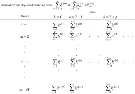
t2t(m1) is the one-step-ahead conditional variance forecast of model m. The estimation steps comprising the SPEC model selection algorithm are summarized in Table 1.The rows of this table refer to candidate ARCH models, the columns refer to trading days, while its entries represent the sums of the squares of the T most recent standardized one-step-ahead prediction errors of each of the M models. Each trading day, the choice of the model to be used to predict the conditional variance for the next day is determined by the entry of the corresponding column of table 1 that has the minimum value. In particular, model
i
m will be chosen at time
k
T
j
if it is the one that corresponds to the cell of columnj
T
that has the minimum value of
j T
j t
i t
r
1 2
Table 1
The estimation steps required at time
k
for each model m by the SPEC model selection algorithm. At timek
(
k
T
,
T
1
,...
), select the model m with the minimum value for the sum of the squares of the T most recent standardized one-step-ahead prediction errors,
k T k t m t t m t t k T k t m t r 1 2 1 | 2 1 | 1
2 ˆ ˆ
ˆ
.Time
Model
k
T
k
T
1
.
.
.
k
T
j
.
.
.
M
m
i
m
m
m
.
.
.
.
.
.
2
1
.
.
.
ˆ
.
.
.
ˆ
ˆ
.
.
.
.
.
.
.
.
.
.
.
.
.
.
.
ˆ
.
.
.
ˆ
ˆ
.
.
.
.
.
.
.
.
.
.
.
.
.
.
.
ˆ
.
.
.
ˆ
ˆ
.
.
.
ˆ
.
.
.
ˆ
ˆ
1 2 1 2 2 1 2 1 2 1 2 2 1 2 1 2 2 1 2 2 2 1 2 2 1 1 2 1 2 1 2 1 1 2
j T j t M t T t M t T t M t j T j t i t T t i t T t i t j T j t t T t t T t t j T j t t T t t T t tr
r
r
r
r
r
r
r
r
r
r
r
4 . E v a l u a t i o n o f V a r i a n c e F o r e c a s t s w i t h S i m u l a t e d O p t i o n P r i c e s
As Engle et al. (1997 p.120) noted, “a natural criterion for choosing between any pair of competing methods to forecast the variance of the rate of return on an asset would be the
expected incremental profit from replacing the lesser forecast with the better one’’. Engle et
independence of the individual forecasts. As a check for the presence of bias, Engle et al. (1993) added the minimum and maximum of the daily forecasts. So, for example, in case of a significant downward bias, the maximum forecast will beat the minimum forecast and all of the individual forecasts that are more severe biased.
The pricing of index options is based on the Black & Scholes option pricing formula (Black and Scholes (1973)). In particular, the forecast price of a call and a put option at time
1
t
given the information available at timet
, with
days to maturity, denoted, respectively, by Ct 1|t and t t
P1| are given by
2 1
|
1 S N d Ke N d
C rft
t t t
,
2 1
|
1 S N d Ke N d
P rft
t t
t
,
where
t t
t t t
t rf
K S
d
| 1
2 | 1
1
2 1 ln
and
d
2
d
1
t 1|t
.Here, St is the market closing price of the stock (or portfolio) at time
t
(used as a forecast for1
t
S ), rft is the daily continuously compounded risk free interest rate andK is the exercise
(or strike) price at maturity day, while,
N
.
and
t 1|t denote, respectively, the cumulativenormal distribution function and the standard deviation of the rate of return during the life of the option, from
t
1
until the maturity day, given the information available at timet
.Each agent applies a variance-forecast method and trades one-day options on a $1 share of the NYSE portfolio. The exercise price is taken to be exp
rft . Thus, for St 1,1
, K exp
rft ,
t t t
t 1|
1 |
1 ˆ
, Ct t Ct 1|t1 |
1
and Pt t Pt 1|t
1 |
1
, the Black & Scholes
option pricing formula reduces to:
0.5ˆ
12 1|
| 1 |
1
t t t t t
t P N
C
.The way in which the simulated options market operates is the following: The daily differences in the variance forecasts of the various methods considered lead to different reservation prices for one-day options on the index considered. These, in turn, trigger option trading among fictitious agents, each using one of the forecast methods considered. A trader with a higher (or lower) variance forecast and, hence, with a higher (or lower) reservation price for the option would buy (or sell) a straddle on a $1 share of index considered from any of the remaining traders with lower (or higher) reservation prices for the option. A straddle option is the purchase (or sale) of both a call and a put option, of the underlying asset, with the same maturity day. The straddle trading is used because a straddle, that has its stock price equal to the exercise price, is Delta neutral. Delta is the change in the option price for a given change in the stock price:
1
0
d
N
e
S
C
CALL
,
and
1
1
0
d
N
e
S
P
PUT
.
The day
t
payoff to agent i from holding the straddle is:
t t t t
t max exp y exp r ,exp r exp y
,
i t t i t t t i t t i t t i t t i t t i t t i t t t i i t C C C C C C C C , | 1 , | 1 1 , | 1 , | 1 , | 1 , | 1 , | 1 , | 1 1 ,1 , for
for ,
-
.In Engle et al. (1993), the GARCH(1,1) forecast method achieves the highest cumulative profits for the three sample lengths. Moreover, the GARCH(1,1) method for a rolling sample of 1000 observations yields the highest profit, dominating even the average of all variance forecast methods.
5 . E v a l u a t i n g t h e S P E C M o d e l S e l e c t i o n A l g o r i t h m o n S i m u l a t e d O p t i o n s
Degiannakis and Xekalaki (2001b) applied a number of statistical evaluation criteria in order to examine the ability of the SPEC model selection algorithm to select the ARCH model that best predicts future volatility, for forecast horizons ranging from one day ahead to one hundred days ahead. Their results showed that the SPEC model selection procedure has a
satisfactory performance in selecting that model that generates “better” volatility predictions.
Moreover, Degiannakis and Xekalaki (2001a) made a comparative study among a set of ARCH model selection algorithms in order to examine which method yields the highest profits in straddle trading based on volatility forecasts using actual option price data. The results showed that the SPEC algorithm for
T
5
achieved the highest rate of return.In the sequel, the performance of the SPEC algorithm as an ARCH model selection criterion is evaluated in the context of a simulated options market in order to avoid biases induced by the use of actual index-option prices. In particular, following Engle et al.’s (1993) approach, an economic criterion to evaluate the SPEC model selection algorithm is adopted: the profit from variance forecasts in pricing one-day index straddle options. A simulated market of option trading among 104 fictitious agents is created, whereby traders use variance forecasts obtained by the models of their choice to price a straddle on the S&P500 index for the next day. The performance of the SPEC algorithm is evaluated through comparing the different volatility forecasts. The comparison is performed on the basis of the cumulative profits of traders each of which always uses volatility forecasts obtained by the same GARCH, EGARCH or TARCH model on the one hand and cumulative profits by traders using volatility forecasts obtained by models suggested by the SPEC criterion on the other.
So, traders can be thought of a having different “methods” or “strategies” for obtaining
variance forecasts (amounting to the utilization of the forecasts of a model at each point in time) and can be classified into two categories: Those who choose to always use one and the same ARCH model and those who at each point in time choose to use the ARCH model suggested by the SPEC algorithm. The variance forecast methods that are compared are: 85
selection “methods” (strategies), one for each of 85 ARCH models, each amounting to the
utilization of the forecasts of the same model at any point in time, the SPEC model selection algorithm for 16 different sample sizes, the average, the minimum and the maximum of all daily forecasts methods.
The data set consists of S&P500 stock index daily returns in the period from June 26th, 1991 to October 18th, 2002, totally 2853 trading days.
The conditional mean is considered as a
th
order autoregressive process:t t t
t z
y
,
1 0 i i t it c c y ,
and
Usually, the conditional mean is either the overall mean or a first order autoregressive process. Theoretically, the
AR
1
process allows for the autocorrelation induced by discontinuous (or non-synchronous) trading in the stocks making up an index (Scholes andWilliams (1977), Lo and MacKinlay (1988)). According to Campbell et al. (1997), “the non -synchronous trading arises when time series, usually asset prices, are taken to be recorded at time intervals of one length when in fact they are recorded at time intervals of other, possible
irregular lengths”. Higher orders of the autoregressive process are considered in order to investigate if they are adequate to produce more accurate predictions.
The conditional variance is regarded as a GARCH(p,q), an EGARCH(p,q) and a TARCH(p,q) function in the forms of (2), (3) and (4), respectively. Thus, the AR(
)GARCH(p,q), AR(
)EGARCH(p,q) and AR(
)TARCH(p,q) models are applied, for
0
,...,
4
,p
0
,
1
,
2
andq
1
,
2
, yielding a total of 85 cases. Numerical maximization of the log-likelihood function, for the E-GARCH(2,2) model, frequently failed to converge. So the five E-GARCH models forp
q
2
were excluded. Maximum likelihood estimates of the parameters are obtained by numerical maximization of the log-likelihood function using the Marquardt algorithm (Marquardt (1963)). The quasi-maximum likelihood estimator (QMLE) is used, as according to Bollerslev and Wooldridge (1992), it is generally consistent, has a limiting normal distribution and provides asymptotic standard errors that are valid under non-normality. The one step-ahead volatility forecasts of the models are:One-step-ahead forecast of the GARCH(p,q) model
p j j t t j q i i t t i t tt
a
a
b
1 2 1 1 2 1 0 2 | 1
ˆ
.One-step-ahead forecast of the EGARCH(p,q) model
p j j t t j qi t i
i t t i i t i t t i t t
t
a
a
b
1 2 1 1 1 1 1 1 0 2 |
1
exp
ln
ˆ
.One-step-ahead forecast of the TARCH(p,q) model
p j j t t j t t t q i i t t i t tt
a
a
D
b
1 2 1 2 1 2 1 0 2 | 1
0
ˆ
.The ARCH processes are estimated using a rolling sample of constant size equal to 1000. Thus, the first one-step-ahead volatility prediction,
ˆt21|t, is available at timet
1000
.Samples of 500 and 2000 observations were also considered leading to similar findings, thus demonstrating that the results of the simulation study are not appreciably affected by the sample size. Tables with the results for rolling samples of 500 and 2000 observations, as well as the full versions of the tables that are presented in the paper for the rolling sample of 1000 observations considered in this section can be found in Degiannakis and Xekalaki (2002).
The SPEC model selection algorithm is applied for various values of T, and, in particular, for
T
5
5
80
. (Here,T
a
b
c
denotesT
a
,
a
b
,
a
2
b
,...,
c
b
,
c
). Thus, based on the SPEC model selection algorithm, sixteen agents are assumed to take part in the simulated options market. Each agent, who follows the SPEC algorithm, selects the ARCH model with the lowest sum of T squared standardized one-step-ahead prediction errors,
Tt1ztt2 1 |
ˆ , in order to forecast next day’s variance. As in Engle et al. (1993), three
more daily forecasts are added: the average of all daily forecasts, the daily minimum and daily maximum forecasts. In the sequel, the resulting forecast methods will be referred to as the AVERAGE, the MINIMUM and the MAXIMUM method, respectively.
days and 104 agents, the
ith
agent’s daily profit per straddle is computed as:
1773 1
103
1 ,
1773 103
t i
i i t
i
[image:11.595.130.466.97.448.2]
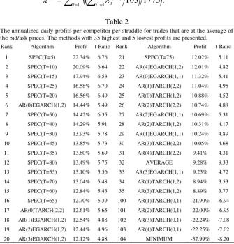
.Table 2
The annualized daily profits per competitor per straddle for trades that are at the average of the bid/ask prices. The methods with 35 highest and 5 lowest profits are presented.
Rank Algorithm Profit t-Ratio Rank Algorithm Profit t-Ratio
1 SPEC(T=5) 22.34% 6.76 21 SPEC(T=75) 12.02% 5.11
2 SPEC(T=10) 20.09% 6.64 22 AR(4)EGARCH(1,2) 12.01% 4.82
3 SPEC(T=15) 17.94% 6.53 23 AR(0)EGARCH(1,1) 11.32% 5.41
4 SPEC(T=25) 16.58% 6.70 24 AR(1)TARCH(2,2) 11.04% 4.95
5 SPEC(T=20) 16.56% 6.49 25 AR(0)TARCH(1,2) 10.88% 4.52
6 AR(0)EGARCH(1,2) 14.44% 5.49 26 AR(2)TARCH(2,2) 10.74% 4.88
7 SPEC(T=50) 14.42% 6.35 27 AR(2)EGARCH(1,1) 10.69% 5.31
8 SPEC(T=40) 14.29% 5.91 28 AR(2)TARCH(1,2) 10.31% 4.17
9 SPEC(T=30) 13.93% 5.78 29 AR(1)EGARCH(1,1) 10.24% 4.89
10 SPEC(T=45) 13.85% 5.73 30 AR(3)TARCH(2,2) 10.05% 4.68
11 SPEC(T=35) 13.80% 5.69 31 AR(4)TARCH(2,2) 9.41% 4.31
12 SPEC(T=80) 13.49% 5.75 32 AVERAGE 9.28% 9.33
13 SPEC(T=55) 13.10% 5.56 33 AR(3)EGARCH(1,1) 9.23% 4.72
14 SPEC(T=70) 13.04% 5.48 34 AR(1)TARCH(1,2) 8.94% 3.53
15 SPEC(T=60) 12.84% 5.43 35 AR(3)TARCH(1,2) 8.89% 3.77
16 SPEC(T=65) 12.70% 5.39 100 AR(1)TARCH(0,1) -21.90% -6.94
17 AR(0)TARCH(2,2) 12.61% 5.65 101 AR(2)TARCH(0,1) -22.00% -6.95 18 AR(1)EGARCH(1,2) 12.54% 4.88 102 AR(3)TARCH(0,1) -22.24% -7.08 19 AR(2)EGARCH(1,2) 12.44% 4.96 103 AR(4)TARCH(0,1) -22.25% -7.02
20 AR(3)EGARCH(1,2) 12.12% 4.88 104 MINIMUM -37.99% -8.20
Any method that yields superior profits relative to the AVERAGE method appears more suitable in predicting volatility for pricing contingent claims. Table 2 presents the profits per competitor per straddle and the corresponding t-ratios (ratio of average daily profit to its standard deviation divided by the square root of the trading days). The methods with the 35 highest and 5 lowest profits are presented. The agents based on the SPEC model selection algorithm clearly outperform the others. All the SPEC model selection based algorithms achieve returns higher than the AVERAGE method. The highest annualized daily returns are achieved by the SPEC(5) model selection algorithm, which is in accordance to Degiannakis and Xekalaki (2001a) results.
which account for recent developments in the area of asset returns volatility, is suggested for further research.
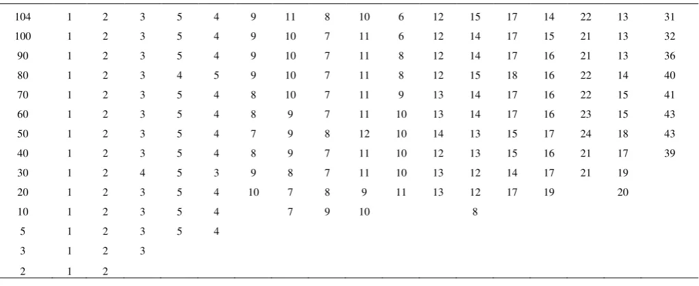
Table 3
Ranks of the methods based on the SPEC model selection algorithm and of the AVERAGE method by dropping out the least profitable agent at a time.
Algorithm
Number of traders
SPEC (T=5)
SPEC (T=10)
SPEC (T=15)
SPEC (T=20)
SPEC (T=25)
SPEC (T=30)
SPEC (T=35)
SPEC (T=40)
SPEC (T=45)
SPEC (T=50)
SPEC (T=55)
SPEC (T=60)
SPEC (T=65)
SPEC (T=70)
SPEC (T=75)
SPEC
(T=80) AVERAGE
104 1 2 3 5 4 9 11 8 10 6 12 15 17 14 22 13 31
100 1 2 3 5 4 9 10 7 11 6 12 14 17 15 21 13 32
90 1 2 3 5 4 9 10 7 11 8 12 14 17 16 21 13 36
80 1 2 3 4 5 9 10 7 11 8 12 15 18 16 22 14 40
70 1 2 3 5 4 8 10 7 11 9 13 14 17 16 22 15 41
60 1 2 3 5 4 8 9 7 11 10 13 14 17 16 23 15 43
50 1 2 3 5 4 7 9 8 12 10 14 13 15 17 24 18 43
40 1 2 3 5 4 8 9 7 11 10 12 13 15 16 21 17 39
30 1 2 4 5 3 9 8 7 11 10 13 12 14 17 21 19
20 1 2 3 5 4 10 7 8 9 11 13 12 17 19 20
10 1 2 3 5 4 7 9 10 8
5 1 2 3 5 4
3 1 2 3
2 1 2
5.1 Ranking of Methods Dropping Out the Least Profitable Agent
An interesting question to investigate is whether the performance of the SPEC algorithm is unaffected by the models that are included in the simulation. This is examined in the sequel by repeatedly running the simulation, each time having dropped out the trader using the least profitable method and calculating the cumulative profits of the remaining participating agents. If the performance of the algorithm is not affected by the models considered, the profits of participants who trade options using the SPEC algorithm should occupy the top places of the ranking. The resulting ranks of the SPEC algorithm based methods and the AVERAGE method are summarized in Table 3. The first column shows the number of participants in each group and the rows present the ranking of the SPEC model selection methods and the AVERAGE method within each group. As there are 104 traders, 103 groups are created, but, for space limitations, only 14 groups are presented. Although there are some slight changes in the rank, the traders based on the SPEC model selection algorithm keep the first places in the ranking. The SPEC(5) model selection algorithm achieves the highest returns in all the cases, thus indicating that the forecasting ability is not sensitive to the models that are used. On the other hand, the AVERAGE method deteriorates as the group becomes smaller. An expected feature as the sample becomes smaller by dropping out the least accurate forecasts.
5.2 Exercise Price and Relative Profits
Following Engle et al.’s (1993) approach, the sensitivity of agents’ profits to exercise
price is examined. Table 4 shows the ranking and cumulative profits of the competitors trading one-day straddles with exercise prices equal to
e
5rft ande
3rft . The call and put
21| 1
21| 1|1| 1|
2 1 2 1
2 2
t
K rf
t t t t t t
t t
t t t t
K rf K rf
C N
e N
,
and
1
1| 1|
1
t
K rf t t t t
P
C
e
, [image:13.595.85.509.221.530.2]for
K
5,
. The rank of the traders does not change significantly. So, the cumulative profits in the simulated market are not sensitive to the exercise price that is used.Table 4. The rank and annualised daily profits of the competitors trading one-day straddles with different exercise prices.
Forecasts
t
rf
e
5e
3rftForecasts
t
rf
e
5e
3rftProfit Rank Profit Rank Profit Rank Profit Rank
SPEC(T=5) 22.46% 1 22.52% 1 SPEC(T=75) 11.88% 22 11.89% 22
SPEC(T=10) 20.29% 2 20.34% 2 AR(4)EGARCH(1,2) 11.94% 21 11.95% 21
SPEC(T=15) 17.84% 3 17.89% 3 AR(0)EGARCH(1,1) 11.15% 23 11.16% 23
SPEC(T=25) 16.50% 4 16.53% 4 AR(1)TARCH(2,2) 11.03% 24 11.03% 24
SPEC(T=20) 16.42% 5 16.46% 5 AR(0)TARCH(1,2) 10.80% 25 10.81% 25
AR(0)EGARCH(1,2) 14.32% 7 14.33% 7 AR(2)TARCH(2,2) 10.79% 26 10.79% 26
SPEC(T=50) 14.40% 6 14.41% 6 AR(2)EGARCH(1,1) 10.52% 27 10.52% 27
SPEC(T=40) 14.21% 8 14.24% 8 AR(2)TARCH(1,2) 10.37% 28 10.37% 28
SPEC(T=30) 13.81% 10 13.84% 9 AR(1)EGARCH(1,1) 10.07% 30 10.07% 30
SPEC(T=45) 13.81% 9 13.83% 10 AR(3)TARCH(2,2) 10.14% 29 10.14% 29
SPEC(T=35) 13.79% 11 13.82% 11 AR(4)TARCH(2,2) 9.50% 31 9.50% 31
SPEC(T=80) 13.34% 13 13.35% 13 AVERAGE 9.46% 32 9.46% 32
SPEC(T=55) 13.41% 12 13.43% 12 AR(3)EGARCH(1,1) 9.12% 33 9.12% 33
SPEC(T=70) 12.89% 14 12.90% 14 AR(1)TARCH(1,2) 8.92% 35 8.93% 35
SPEC(T=60) 12.83% 15 12.85% 15 AR(3)TARCH(1,2) 8.99% 34 8.98% 34
SPEC(T=65) 12.55% 17 12.56% 17 AR(1)TARCH(0,1) -22.06% 100 -22.08% 100
AR(0)TARCH(2,2) 12.69% 16 12.70% 16 AR(2)TARCH(0,1) -22.13% 101 -22.15% 101
AR(1)EGARCH(1,2) 12.38% 18 12.39% 18 AR(3)TARCH(0,1) -22.38% 102 -22.40% 102
AR(2)EGARCH(1,2) 12.32% 19 12.33% 19 AR(4)TARCH(0,1) -22.39% 103 -22.42% 103
AR(3)EGARCH(1,2) 12.03% 20 12.04% 20 MINIMUM -38.14% 104 -38.24% 104
6 . C o m p a r i n g M e t h o d s o f M o d e l S e l e c t i o n o n S i m u l a t e d O p t i o n s
The selection of the appropriate model is one of the most challenging areas in statistical modeling. Usually, a researcher has to choose among a set of candidate models. Methods of model selection examine the ability of the models either to describe or to forecast the variable under investigation. The Akaike information criterion (Akaike (1973)) and the Schwarz Bayesian criterion (Schwarz (1978)) are model selection methods that are based on the maximized value of the log-likelihood function and evaluate the ability of the models to describe the data. In the case we are interesting in using a model for forecasting, the evaluation of the models would naturally be based on their ability to produce valuable forecasts. Loss functions, which measure either the distance between actual and predicted values or the benefit from the use of these forecasts, are used to evaluate the forecasting ability of the models. Poon and Granger (2003) reviewed a detailed record of volatility forecasting loss functions and relative references.
profits of the participants in a simulated options market. Denoting the realized at time
t
1
by2 1
t
s
, the following loss functions were considered: 1. Mean Square Error of Variance (MSEV):
T
t t t t s T 1 2 2 1 2 | 1
1
ˆ.
2. Mean Absolute Error of Variance (MAEV):
T
t t t t s T 1 2 1 2 | 1
1
ˆ.
3. Mean Square Error of Deviation (MSED):
T
t t t t s T 1 2 1 | 1
1
ˆ.
4. Mean Absolute Error of Deviation (MAED):
T
t t t t s T 1 1 | 1
1
ˆ.
5. Heteroscedasticity Adjusted Mean Squared Error of Variance (HAMSEV):
T
t t t t s T 1 2 2 | 1 2 1 1 ˆ
1
.6. Heteroscedasticity Adjusted Mean Absolute Error of Variance (HAMAEV):
T
t t t t s T 1 2 | 1 2 1 1 ˆ
1
.7. Heteroscedasticity Adjusted Mean Squared Error of Deviation (HAMSED):
T
t t t t s T 1 2 | 1 1 1 ˆ
1
.8. Heteroscedasticity Adjusted Mean Absolute Error of Deviation (HAMAED):
T
t t t t s T 1 | 1 1 1 ˆ
1
.9. Mean Logarithmic Error of Variance (MLEV):
T t t t t s T 1 2 2 | 1 2 1 1 ˆln
.10. Gaussian Maximum Likelihood Error of Variance (GMLEV):
Tt t t
t t t s T 1 2 | 1 2 1 2 | 1 1 ˆ ˆ ln
.11. Gaussian Maximum Likelihood Error of Deviation (GMLED):
Tt t t
t t t
s T
1 1|
1 | 1 1 ˆ ˆ ln
,where T is the number of the one-step-ahead volatility forecasts. The first four loss functions have been widely used in applied studies. The heteroscedasticity adjusted functions were introduced by Andersen et al. (1999) and Bollerslev and Ghysels (1996), while mean logarithmic error function was utilized by Pagan and Schwert (1990). The GMLE function, which was presented in Bollerslev et al. (1994), measure the forecast error according to the likelihood function that is used in estimating the models.
the realized intra-day volatility, the interested reader is referred to Andersen et al. (2003) and Andersen et al. (2004). Based on Andersen et al. (1999), Andersen et al. (2001) and Kayahan et al. (2002), we compute the realized intra-day volatility of day
t
as:
1
1
2 , ,
1 2
ln ln
m
j
t m j t
m j
t P P
s ,
where
P
m,t denotes five-minute linearly interpolated prices of S&P500 at dayt
with mobservations per day. The intra-day quotation data are available from April 28th 1997 to October 18th 2002 and were provided by Olsen and Associates.
Each loss function is computed for
T
10
10
80
. In order to compare the SPEC algorithm with the 11 loss functions, a simulated options market is created. Each agent selectsthe ARCH model with the lowest value of its the loss function in order to forecast next day’s
variance. The simulated market is consisting of 99 traders: the 12 model selection algorithms for 8 different sample sizes (including the SPEC algorithm), the average, the minimum and the maximum of all daily forecasts methods. The comparison is carried out on the basis of the annualized daily profits of the participants.
The resulting ranking of the criteria is summarized in Table 5 (Columns 1 and 2). For each model selection criterion, the highest annualized daily profits are given (column 3) along with the values of the corresponding t-ratios (column 4) defined as in Table 2 and the sample sizes (values of T) at which the maximum returns are attained (in parentheses in column 2). (The full table referring to the profits of the 99 traders can be found in Xekalaki and Degiannakis (2004)).
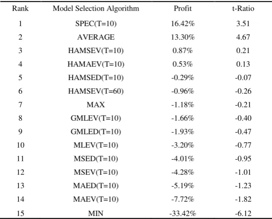
[image:15.595.159.436.490.713.2]The results in the table indicate that traders who are based on the SPEC algorithm achieve the highest returns, despite the use of the realized intra-day volatility by the loss functions. Moreover, the SPEC method appears more suitable in predicting volatility for pricing contingent claims, as it is the only model selection method that produces returns higher that the AVERAGE algorithm does. An interesting point is that, with the exception of HAMSEV, all the algorithms achieve their highest returns for
T
10
.Table 5
The annualised daily profits per competitor per straddle for trades that are at the average of the bid/ask prices.
Rank Model Selection Algorithm Profit t-Ratio
1 SPEC(T=10) 16.42% 3.51
2 AVERAGE 13.30% 4.67
3 HAMSEV(T=10) 0.87% 0.21
4 HAMAEV(T=10) 0.53% 0.13
5 HAMSED(T=10) -0.29% -0.07
6 HAMSEV(T=60) -0.96% -0.26
7 MAX -1.18% -0.21
8 GMLEV(T=10) -1.66% -0.40
9 GMLED(T=10) -1.93% -0.47
10 MLEV(T=10) -3.20% -0.77
11 MSED(T=10) -4.01% -0.95
12 MSEV(T=10) -4.28% -1.01
13 MAED(T=10) -5.19% -1.23
14 MAEV(T=10) -7.72% -1.82
7 . D i s c u s s i o n
Adopting Engle et al.’s (1993) approach to comparing several variance forecast
methods using an economic value criterion, the performance of the SPEC model selection algorithm was examined. Simulating an options market, in order to avoid problems related to observed actual option prices, 104 traders were assumed to trade one-day straddles on $1 shares of the S&P500 index, for the period from October 4th 1995 to October 18th, 2002 (1773 trading days). Traders were also assumed to use variance forecast methods of their choice. The variance forecast methods considered were: 85
selection “methods”
(strategies), one for each of 85 ARCH models, each amounting to the utilization of the
forecasts of the same model at any point in time, the SPEC model selection algorithm
for 16 different sample sizes, the average, the minimum and the maximum of all daily
forecasts methods. Traders using SPEC algorithm based methods appear to achieve
higher profits than traders using any of the 85 single ARCH model based methods
considered in the simulation.
Moreover, traders, who apply the SPEC model selection algorithm for sample sizesT
5
5
2
5
, appear to achieve the highest profits, a conclusionwhich is in agreement to Degiannakis and Xekalaki’s (2001a) findings in the case of real index-option prices. The ability of the SPEC model selection algorithm was also compared with loss functions that measure the ability of the models to forecast volatility. Even though, the other criteria (loss functions) used the realized intra-day volatility, the SPEC algorithm, for
T
10
, led to the highest profits. It appears, therefore, that the results support the conclusion that the increase in profits cannot be attributed to chance but to improved volatility prediction. Hence, the SPEC selection method offers a useful model selection tool in estimating future volatility, with applications in pricing derivatives.R e f e r e n c e s
Akaike, H., 1973. Information Theory and the Extension of the Maximum Likelihood Principle. Proceeding of the Second International Symposium on Information Theory. Budapest, 267-281.
Andersen, T.G. and Bollerslev, T., 1998. Answering the Skeptics: Yes, Standard Volatility Models Do Provide Accurate Forecasts. International Economic Review, 39, 885-905. Andersen, T.G., Bollerslev, T. and Lange, S. 1999. Forecasting Financial Market Volatility:
Sample Frequency vis-à-vis Forecast Horizon. Journal of Empirical Finance, 6, 457-477. Andersen, T.G., Bollerslev, T., Diebold, F.X. and Ebens H., 2001. The Distribution of Stock
Return Volatility. Journal of Financial Economics, 61, 43-76.
Andersen, T.G., Bollerslev, T., Diebold, F.X. and Labys, P., 2003. Modeling and Forecasting Realized Volatility. Econometrica, 71, 529-626.
Andersen, T.G., Bollerslev, T. and Diebold, F.X., 2004. Parametric and Nonparametric Volatility Measurement. Handbook of Financial Econometrics, (eds.) Yacine Aït-Sahalia and Lars Peter Hansen, Amsterdam, North Holland, forthcoming.
Bera, A.K. and Higgins, M.L., 1993. ARCH Models: Properties, Estimation and Testing. Journal of Economic Surveys, 7, 305-366.
Black, F., 1976. Studies of Stock Market Volatility Changes. Proceedings of the American Statistical Association, Business and Economic Statistics Section, 177-181.
Black, F. and Scholes, M., 1973. The Pricing of Options and Corporate Liabilities. Journal of Political Economy, 81, 637-654.
Bollerslev, T., 1986. Generalized Autoregressive Conditional Heteroscedasticity. Journal of Econometrics, 31, 307-327.
Bollerslev, T. and Ghysels, E., 1996. Periodic Autoregressive Conditional Heteroskedasticity, Journal of Business and Economic Statistics, 14, 139-157.
Bollerslev, T. and Wooldridge, J., 1992. Quasi-Maximum Likelihood Estimation and Inference in Dynamic Models with Time Varying Covariances. Econometric Reviews, 11, 143-172.
Bollerslev, T., Chou, R.C. and Kroner, K., 1992. ARCH Modelling in Finance: A Review of the Theory and Empirical Evidence. Journal of Econometrics, 52, 5-59.
Bollerslev, T., Engle, R.F. and Nelson, D., 1994. ARCH Models. In R.F. Engle and D.L. McFadden (Ed.), Handbook of Econometrics, Ch.49, IV Elsevier.
Box, G.E.P. and Tiao, G.C., 1973. Bayesian Inference in Statistical Analysis. Reading, Mass. Cai, J., 1994. A Markov Model of Switching-Regime ARCH. Journal of Business and
Economic Statistics, 12, 309-316.
Campbell, J., Lo, A. and MacKinlay, A.C., 1997. The Econometrics of Financial Markets. New Jersey, Princeton University Press.
Degiannakis, S. and Xekalaki, E., 1999. Predictability and Model Selection in the Context of ARCH Models. Technical Report no 69, Department of Statistics, Athens University of Economics and Business. (http://stat-athens.aueb.gr/~exek/papers/Xekalaki-TechnRep69(1999)ft.pdf).
Degiannakis, S. and Xekalaki, E., 2001a. Using a Prediction Error Criterion for Model Selection in Forecasting Option Prices. Technical Report no 131, Department of Statistics, Athens University of Economics and Business. (http://stat-athens.aueb.gr/~exek/papers/Xekalaki-TechnRep131(2001a)ft.pdf).
Degiannakis, S. and Xekalaki, E., 2001b. Assessing the Performance of a Prediction Error Criterion Model Selection Algorithm. Technical Report no 133, Department of Statistics, Athens University of Economics and Business. (http://stat-athens.aueb.gr/~exek/papers/Xekalaki-TechnRep133(2001b)ft.pdf).
Degiannakis, S. and Xekalaki, E., 2002. Using the Prediction Error Criterion as a Selection Method in Forecasting Option Prices: A Simulation Approach. Technical Report no 191, Department of Statistics, Athens University of Economics and Business. (http://stat-athens.aueb.gr/~exek/papers/Xekalaki-TechnRep191(2002)ft.pdf)
Degiannakis, S. and Xekalaki, E., 2004. Autoregressive Conditional Heteroscedasticity Models: A Review. Quality Technology and Quantitative Management, 1(2). (In press) Ding, Z., Granger, C.W.J. and Engle, R.F., 1993. A Long Memory Property of Stock Market
Returns and a New Model. Journal of Empirical Finance, 1, 83-106.
Engle, R.F., 1982. Autoregressive Conditional Heteroscedasticity with Estimates of the Variance of the United Kingdom Inflation. Econometrica, 50(4), 987-1007.
Engle, R.F. and Ng, V.K., 1993. Measuring and Testing the Impact of News on Volatility. Journal of Finance, 48, 1749-1778.
Engle, R.F., Hong, C.H., Kane, A. and Noh, J., 1993. Arbitrage Valuation of Variance Forecasts with Simulated Options. Advances in Futures and Options Research, 6, 393-415.
Engle, R.F., Kane, A. and Noh, J., 1997. Index-Option Pricing with Stochastic Volatility and the Value of the Accurate Variance Forecasts. Review of Derivatives Research, 1, 120-144.
Giot, P. and Laurent, S., 2003. Value-at-Risk for Long and Short Trading Positions. Journal of Applied Econometrics, 18, 641-664.
Glosten, L.R., Jagannathan, R. and Runkle, D.E., 1993. On the relation between the expected value and the volatility of the nominal excess return on stocks. Journal of Finance, 48, 1779-1801.
Gourieroux, C., 1997. ARCH models and Financial Applications. Springer Series.
Hamilton, J.D. and Susmel, R., (1994). Autoregressive Conditional Heteroskedasticity and Changes in Regime. Journal of Econometrics, 64, 307-333.
Harvey, A.C., 1981. The Econometric Analysis of Time Series. Oxford.
Hsieh, D.A., 1989. Modeling Heteroscedasticity in Daily Foreign-Exchange Rates. Journal of Business and Economic Statistics, 7, 307-317.
Jorion, P., 1988. On Jump Processes in the Foreign Exchange and Stock Markets. Review of Financial Studies, 1, 427-445.
Kane, A. and Marks, S.G., 1987. The Rocking Horse Analyst. Journal of Portfolio Management, 13, 32-37.
Kayahan B., Saltoglu, T. and Stengos, T., 2002. Intra-Day Features of Realized Volatility: Evidence from an Emerging Market. International Journal of Business and Economics, 1(1), 17-24.
Lambert, P. and Laurent, S., 2000. Modeling Skewness Dynamics in Series of Financial Data. Discussion Paper. (Institut de Statistique, Louvain-la-Neuve).
Lambert, P. and Laurent, S., 2001. Modeling Financial Time Series Using GARCH-Type Models and a Skewed Student Density. Mimeo. (Universite de Liege).
Lo, A. and MacKinlay, C., 1988. Stock market prices do not follow random walks: Evidence from a simple specification test. Review of financial studies, 1, 41-66.
Mandelbrot, B., 1963. The variation of certain speculative prices. Journal of Business, 36, 394-419.
Marquardt, D.W., 1963. An Algorithm for Least Squares Estimation of Nonlinear Parameters. Journal of the Society for Industrial and Applied Mathematics, 11, 431-441.
Nelson, D.B., 1991. Conditional Heteroscedasticity in Asset Returns: A New Approach. Econometrica, 59, 347-370.
Pagan, A.R. and Schwert, G.W., 1990. Alternative Models for Conditional Stock Volatility. Journal of Econometrics, 45, 267-290.
Poon, S.H. and Granger, C.W.J., 2003. Forecasting Volatility in Financial Markets: A Review, Journal of Economic Literature, XLI, 478-539.
Scholes, M. and Williams, J., 1977. Estimating betas from nonsynchronous data. Journal of Financial Economics, 5, 309-327.
Schwarz, G., 1978. Estimating the Dimension of a Model. Annals of Statistics, 6, 461-464. Sentana, E., 1995. Quadratic ARCH models. Review of Economic Studies, 62, 639-661. Vilasuso, J., 2002. Forecasting Exchange Rate Volatility. Economics Letters, 76, 59-64. Xekalaki, E. and Degiannakis, S, 2004. A Comparison of the Standardized Prediction Error
Criterion with Other ARCH Model Selection Criteria. Technical Report no 205, Department of Statistics, Athens University of Economics and Business. (http://stat-athens.aueb.gr/~exek/papers/Xekalaki-TechnRep205(2004)ft.pdf)
Xekalaki E., Panaretos, J. and Psarakis, S., 2003. A Predictive Model Evaluation and Selection Approach - The Correlated Gamma Ratio Distribution. In: J. Panaretos (Ed.), Stochastic Musings: Perspectives from the Pioneers of the Late 20th Century, Lawrence Erlbaum Associates Publishers, 188-202.