Fault Detection and Classification using Kalman Filter
and Hybrid Neuro-Fuzzy Systems
A. Khoukhi
Dept. Systems Engineering
KFUPM Dhahran, KSA, 31261
H. Khalid
R. Doraiswami
Dept. Systems Dept. Systems Engineering Engineering KFUPM KFUPM Dhahran, Dhahran, KSA, 31261 KSA, 31261
L. Cheded
Dept. Systems Engineering
KFUPM Dhahran, KSA, 31261
ABSTRACT
In this paper, an efficient scheme to detect and classify faults in a system using kalman filtering and hybrid neuro-fuzzy computing techniques, respectively, is proposed. A fault is detected whenever the moving average of the Kalman filter residual exceeds a threshold value. The fault classification has been made effective by implementing a hybrid neuro-fuzzy Inference system. By doing so, the critical information about the presence or absence of a fault is gained in the shortest possible time, with not only confirmation of the findings but also an accurate unfolding-in-time of the finer details of the fault, thus completing the overall fault diagnosis picture of the system under test. The proposed scheme is evaluated extensively on a two-tank process used in industry exemplified by a benchmarked laboratory scale coupled-tank system.
Keywords
Kalman filter, soft computing, ANN, genetic algorithm, ANFIS, fault detection, fault isolation, benchmarked laboratory scale two-tank systems
1.
INTRODUCTION
Challenging design problems arise in modern fault diagnosis systems. Unfortunately, the classical analytical techniques often cannot provide acceptable solutions to such difficult tasks. This explains why soft computing techniques such as fuzzy logic, neural networks and evolutionary algorithm have become more and more popular in industrial applications of fault diagnosis. Process faults, if undetected, have a serious impact on process operation and efficiency, product quality, safety, productivity and pollution level. In order to detect, diagnose and correct these abnormal process behaviors, the use of efficient and advanced automated diagnostic systems is of great importance to modern industries. The main objective of fault detection and isolation (FDI) is to provide early warnings to operators, such that appropriate actions can be taken to prevent the breakdown of the system caused by the occurrence of faults. This will improve the reliability and safety of the system, and avoid unnecessary and costly downtimes. Complete reliance on human operators to monitor the conditions of the systems is often difficult, especially as engineering systems are becoming ever more complex.
For example, in chemical processes, several kinds of failures may compromise safety and productivity. In fact, the occurrence of faults may reduce the efficiency of the process (e.g., lower product quality) or, in the worst scenarios, could lead to fatal accidents (e.g., temperature run-away) leading to injuries to personnel, environmental pollution and equipment damage. Major failures to be considered in chemical processes are: actuator failures (e.g., electric-power failures, pump failures, valves failures), process failures (e.g., abrupt variations of some process parameters, side reactions due to impurities in the raw materials) and sensor failures. To tackle these difficulties, Fault Diagnosis and Isolation (FDI) techniques need to be developed.
The model-based approach is popular for developing FDI techniques [1][2]. It mainly consists of two stages [3]. The first one is to generate residuals by computing the difference between the measured output and the estimated output obtained from the model of the system. Any departure of the residuals from zero indicates that a fault has likely occurred [4]. However, these methods are developed mainly for linear systems assuming that a precise mathematical model of the system is available. This assumption, however, may be difficult to satisfy in practice, especially as engineering systems are becoming more complex and are in general nonlinear [5][6]. Several model-based studies on the detection and identification of faults and tuning parameters were considered in [7-8].
The paper is organized as follows: Section II reviews some related studies in this area, whereas Section III states the fault diagnosis problem at hand. Section IV discusses the implementation and simulation results. Finally some conclusions are given Section V.
2.
OVERVIEW OF FDI TECHNIQUES
of the work on quantitative model-based approaches has been based on using general input-output and state space models to generate residuals. These approaches can be classified into observer/filter-based, parity space and frequency domain methods. Good survey papers include [9-13]. The mathematical model-based approach adopted in this paper falls into the observer category. The basic idea behind the observer- or filter-based approaches is to estimate the outputs of the system from the measurements (or a subset of measurements) by using either observers in a deterministic setting or statistical filters (e.g. the Kalman filter) in a stochastic setting. Then, the weighted output estimation errors (or innovations in the stochastic case) are used as the residuals. Depending on the circumstances, one may use linear or nonlinear, full or reduced-order, fixed or adaptive observers (or Kalman filters) in the generation of residuals.
Soft computing techniques are used to develop models required in FDI. Through the use of expert knowledge, rules and training, these techniques can provide models for a wide class of nonlinear systems with arbitrary accuracy. Among these techniques, neural networks are well recognized for their learning ability which allows them to approximate a wide class of nonlinear functions with an arbitrary accuracy [14]. For these reasons, they have been applied to many engineering problems [15-18], and used as models to generate residuals for fault detection [19]. However, these networks are inadequate in isolating faults, as they are black boxes in nature. Further, it is also desirable that a fault diagnostic system should be able to incorporate the experience of the operators [20] which cannot completely represented by a dynamical model. Fuzzy reasoning allows symbolic generalization of numerical data by fuzzy rules and supports the direct integration of the experience of the operators in the decision-making process of FDI in order to achieve a more reliable fault diagnosis [21]. An up-to-date application of FDI techniques to motor fault detection and isolation was recently published in a special section in [22]. In what follows, a brief literature review is presented under three sections comprising of fault diagnosis using expert systems, fuzzy logic, neural network and Genetic Algorithm.
In recent years, the application of fuzzy logic to model-based fault diagnosis has gained increasing attention in both fundamental research and application. Rule-based feature extraction has been widely used in expert systems for many applications. Initial attempts at the application of expert systems for fault diagnosis can be found in the work of Henley [23] and Niida [24]. Structuring the knowledge-base through hierarchical classification can be found in [25]. Ideas on knowledge-based diagnostic systems based on the task framework can be found in [26]. A rule-based expert system for fault diagnosis in a cracker unit is described in [27]. More work on expert systems in chemical process fault diagnosis can be found in [28] and [29]. Wo et al. [30] presented an expert fault diagnostic system that uses rules with certainty factors. Leung and Romagnoli [31] presented a probabilistic model-based expert system for fault diagnosis. An expert
system approach for fault diagnosis in batch processes was also discussed in Scenna [32]. Expert systems posses attractive features as they are knowledge based systems generated using input/output data and an inference engine built upon a set of rules defined by experts in the problem field. Nevertheless, major drawbacks of these systems include adaptivity to new and changing environment, the increasing of the number of rules.
Soft computing have been seen by many researchers as an alternative to classical expert systems paradigm, and a considerable interest was shown in the literature regarding the application of soft computing to fault diagnosis. A number of papers address the problem of fault diagnosis using back-propagation neural networks.
In chemical engineering, Watanabe et al. [33], Venkatasubramanian and Chan [34], Ungar et al. [35] and Hoskins et al. [36] were among the first researchers to demonstrate the usefulness of neural networks for fault diagnosis. A detailed and thorough analysis of neural networks for fault diagnosis in steady-state processes was presented by Venkatasubramanian et al. [37]. This work was later extended to utilize dynamic process data by Vaidyanathan and Venkatasubramanian [38]. A hierarchical neural network architecture for the detection of multiple faults was proposed by Watanabe et al. [39]. Most of the work on the improvement of the performance of standard back-propagation neural networks for fault diagnosis is based on the idea of explicit feature presentation to the neural networks by Fan et al. [40], Farell and Roat [41], Tsai and Chang [42], and Maki and Loparo [43]. Modifications to the selection of basis functions have also been suggested to the standard back-propagation network with a view to improving both the accuracy and training time. For example, Leonard and Kramer [44] suggested the use of radial basis function networks for fault diagnosis applications.
Genetic Algorithms (GAs) have been implemented for a wide variety of problems, both real-world (e.g. fault diagnosis and fault tolerant systems) and abstract (e.g. solving NP-complete problems [45]). The bulk of the GA literature is concerned with practical applications. For a very complete bibliography, see [46], which contains a comprehensive survey.
3.
THE FAULT DIAGNOSIS PROBLEM
STATEMENT
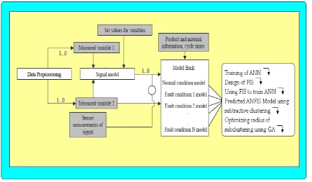
[image:3.595.56.279.219.349.2]Fault is an undesirable factor in any process control industry. It affects the efficiency of system operation and reduces economic benefit to the industry. The early detection and diagnosis of faults in mission critical systems becomes highly crucial for preventing failure of equipment, loss of productivity and profits, management of assets, reduction of shutdowns. To have an effective fault diagnosis of highly non-linear systems, hybrid techniques have been utilized here in the proposed genetic neuro-fuzzy Based- FDI.
Fig 1: Implementation plan for the evaluation of the proposed scheme
3.1
System Description
The Benchmarked laboratory-scale process control system was used to collect data. The data was collected at a sampling time of 50 milliseconds. Different data sets were generated for the PI-based water level control system. Different fault scenarios were also been considered for the generation of the data sets.
The proposed scheme was evaluated on the above- cited process control system. The scheme is carried out by jointly interpreting model outputs. The implementation plan for the proposed scheme is shown in the Figure 1.
3.2
Experimental Setup
The process Data was generated through an experimental setup as shown in Figure 2. A two-tank system was used in order to collect the data with the introduction of actuator, and sensor faults through the system as can be seen in the labview circuit window. An amplified voltage of 18 volts was used to handle the controller effectively for the changes/fluctuations produced in the system. So, the fault diagnosis was done here in a closed-loop identification setup where the controller tends to suppress the faults while it is performing its feedback control task.
3.3
Process Data Collection and
Description
The process data was collected at 50-millisecond sampling time. The main objective of the benchmarked dual-tank system is to reach a reference height of 200 ml in the second tank. During this process, several faults were introduced such as leakage faults, sensor faults and actuator faults. Leakage faults were introduced through the pipe clogs of the system,
knobs between the first and the second tank, etc. Sensor faults were simulated by introducing a gain in the circuit as if there was a fault in the level sensor of the tank. Actuator faults were simulated by introducing a gain in the setup for the actuator that comprises of the motor and pump. A PI controller was employed in order to reach the desired reference height. Due to the inclusion of faults, the controller was finding it difficult to reach the desired level. For this reason, the power of the motor was increased from 5 volts to 18 volts in order to provide it with the maximum throttle to reach the desired level. In doing so, the actuator performed well in achieving its desired level but it also suppressed the faults of the system. So, it made the task of detecting the faults. After the collection of data, techniques of estimating key parameters such as settling time, steady- state value, and coherence spectra can be used to help us get a useful insight into the fault.
3.4
D. Model of the Coupled Tank System
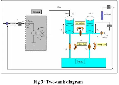
The physical system under evaluation is formed of two tanks connected by a pipe. The leakage is simulated in the tank by opening the drain valve. A DC motor-driven pump supplies the fluid to the first tank and a PI controller is used to control the fluid level in the second tank by maintaining the level at a specified level, as shown in Figure 3. A step input is applied to the dc motor- pump system to fill the first tank. The opening of the drainage valve introduces a leakage in the tank. Various types of leakage faults are accompanied with a more detailed fault picture. The National Instruments LABVIEW package is employed to collect these data.
(a)
(b)
Fig 2: (a) The two tank system with the Labview with a DAQ and the amplifier for the magnified voltage
[image:3.595.315.539.435.718.2]Firstly, the data collected from the plant has been normalized which comprises of the pre-processing of the data. Then, the optimal cluster has been tested through ANFIS using the subtractive clustering technique. Then, the genetic optimization of the subtractive clustering radius has been performed and the performance has been validated by checking the root-mean square error and the performance targets.
Fig 3: Two-tank diagram
4.
IMPLEMENTATION AND
SIMULATION RESULTS
The model of the system for a fault-free, which is obtained from the system identification process described in the previous section, is given by:
0 0
(
1)
( )
(
)
( )
x k
+
=
A x k
+
B u k
-
d
+
w k
(1)0
( )
( )
( )
y k
=
C x k
+
u
k
zero-mean white plant and measurement noise signals, respectively, with covariance’s:
( )
T( )
Q
=
E w k w k
é
ë
ù
û
, and R= E v k v kéë( ) T( )ùû (2)The plant noise,
w k
( )
, is a mathematical artifice introduced to account for the uncertainty in the a-priori knowledge of the plant model. The larger the covariance Q is, the less accurate the model(
A B C
0,
0,
0)
is and vice versa. The Kalman filteris given by:
(
)
0 0 0 0
ˆ
(
1)
ˆ
( )
(
)
( )
ˆ
( )
x k
+
=
A x k
+
B u k
-
d
+
K y k
-
C x k
(3)0
ˆ
( )
( )
( )
e k
=
y k
-
C x k
where
d
is the delay and e (k) the residual, K0 is the filtergain. The larger the Kalman filter gain K0is, the faster the
response of the filter will be and the larger the variance of the estimation error becomes. Thus, there is a trade-off between a fast filter response and a small covariance of the residual. An adaptive on-line scheme is employed to tweak the a- priori choice of the covariance matrices so that an acceptable trade-off between the Kalman filter performance and the covariance of the residual is reached. Appendix 1 gives the full details of the mathematical model, including the linearized version, of the dual-tank process. A PI controller, with gains
k
pandk
I, is used to maintain the level of the Tank 2 at the desired reference inputr
.It is worth pointing out here that the fault-free model of the system is identified using a recursive least-squares
identification scheme. The order of the estimated model was iterated to obtain an acceptable model structure using a combination of the AIC criterion and the identified pole locations. The identified model is essentially a second-order system with a delay even though the theoretical model is of a fourth order. Using the fault-free model together with the covariance of the measurement noise, R, and the plant noise covariance, Q, the Kalman filter model was finally derived. As it is difficult to obtain an estimate of the plant covariance, Q, a number of experiments were performed under different plant scenarios to tune the Kalman gain,K0
(
)
0 0 0 0
ˆ
(
1)
ˆ
( )
(
)
( )
ˆ
( )
x k
+
=
A x k
+
B u k
-
d
+
K
y k
-
C x k
(4)0
ˆ
( )
( )
( )
e k
=
y k
-
C x k
The Kalman filter was evaluated under different fault scenarios for an on-off controller, a P controller, and a PI controller, as shown in Figure 4.
4.1
ANN-Based Fault Diagnosis
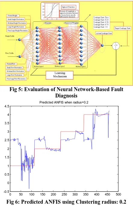
The analysis of the ANN is a difficult task and it requires a wide experience in selecting the training sets, activation functions and the number and size of the hidden layers for the application at hand. A generic model of the ANN in fault diagnosis is as shown in Figure 5.
4.2
Subtractive Clustering ANFIS-Based
Fault Diagnosis
0 500 1000 1500 2000 2500 0 50 100 150 200 time h e ig h t
The height profile and the residual of Kalman filter
0 500 1000 1500 2000 2500 -10 -5 0 5 time re s id u a l residual (a)
0 50 100 150 200 250 300 350 0 100 200 300 time h e ig h ts
heights for fault-free and faulty cases
[image:5.595.318.539.71.414.2]0 50 100 150 200 250 300 350 -2 0 2 4 6 residual time re s id u a l (b)
Fig 4: Kalman filter results for an (a) On-Off and (b) PI Controller: for Flow and Height under various leakage
magnitudes
The green graph shows the prediction with the subtractive clustering technique followed the blue graph in each of all the four phases which is showing the genetic optimization of the radius parameter of the sub-clustering technique. When implemented in the genetic algorithm, these functions give the best fitness function value as follows: Fitness Function Value:0.187462
4.3
Discussion
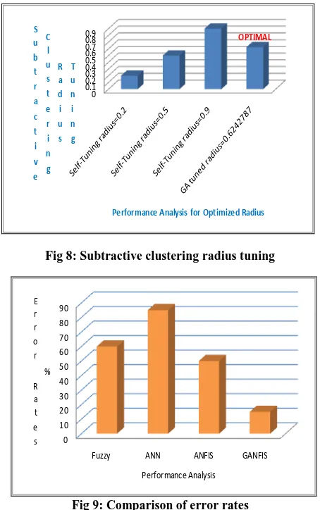
In this paper, a hybrid FDI scheme, involving a model-based kalman filter approach and a model-free genetic neuro-fuzzy approach, was proposed and evaluated on a lab-scale benchmarked process control system exemplified by a two-tank system.. A good comparison of the techniques can be seen in the histograms shown in Figures 6 and 7. In Figure 8, it can be seen, that when the radius of the subtractive clustering is chosen randomly, it leads to improvements in the results. The chart in Figure 9 shows the comparison with the error rates between fuzzy, ANN, ANFIS and the proposed genetic neuro-fuzzy method. It is important to note here that the error rate for the GANFIS is the least one because the genetic algorithm has well performed in the optimization of the subtractive clustering. Further research is also ongoing in optimizing the ANN and FIS structures.
[image:5.595.55.272.71.438.2]Fig 5: Evaluation of Neural Network-Based Fault Diagnosis
Fig 6: Predicted ANFIS using Clustering radius: 0.2
0 50 100 150 200 250 300 350 400 450 500 0 0.5 1 1.5 2 2.5 3 3.5 4 4.5 5 Fault-Level Prediction Data Points 1 : S m a ll Fa u lt , 2 : M e d . Fa u lt , 3 : L a rg e Fa u lt , 4 : N o -Fa u lt Original Predicted ANFIS Predicted GANFIS (a)
0 50 100 150 200 250 300 350 400 450 500 1 1.5 2 2.5 3 3.5 4 4.5 5
Phase # 2: Fault-Level Prediction - Predicted Sub-Clustered ANFIS with GA
Data Points 1 : S m a ll Fa u lt , 2 : M e d . Fa u lt , 3 : L a rg e Fa u lt , 4 : N o -Fa u lt Original
Predicted Sub-Clust ANFIS Predicted ANFIS with GA
[image:5.595.321.529.75.745.2](b)
Fig 7: Various Fault level Prediction through 2 phases
0 50 100 150 200 250 300 350 400 450 500
-0.5 0 0.5 1 1.5 2 2.5 3 3.5 4 4.5
[image:5.595.329.527.424.755.2]0 0.1 0.2 0.3 0.4 0.5 0.6 0.7 0.8 0.9 OPTIMAL S u b t r a c t i v e C l u s t e r i n g R a d i u s T u n i n g
[image:6.595.53.280.69.431.2]Performance Analysis for Optimized Radius
Fig 8: Subtractive clustering radius tuning
0 10 20 30 40 50 60 70 80 90
Fuzzy ANN ANFIS GANFIS E r r o r R a t e s % Performance Analysis
Fig 9: Comparison of error rates
5.
CONCLUSION
In this paper, we presented a model-free approach to the fault diagnosis problem, based on a combination of different learning strategies like ANN, adaptive neuro-fuzzy and ANFIS. This model-free approach detects a presence of a possible fault from the profiles of the sensor outputs. Changes in the fault signatures such as settling time, and the steady-state value, give a quick indication that a fault may be in the making. An abrupt change in the sensor output profile indicates a possible onset of a fault. As such, this model-free approach can be made an effective part of an overall integrated approach that tackles both fault detection and isolation where the isolation part would be handled by an additional section using a model-based approach.
6.
ACKNOWLEDGMENT
The authors wish to acknowledge the support of KFUPM in carrying out this work under the grant of IN1011027.
7.
APPENDIX
The mathematical model of a benchmark model of a cascade connection of a dc motor and a pump relating the input to the motor, u, and the flow,
Q
i, is a first-order system :( )
i m i m
Q
a Q
b
u
(A1) Four random Phases for trained subcluster ANFIS with GAwhere
a
mandb
mare the parameters of the motor-pump system and
( )
u
is a dead-band and saturation type of nonlinearity. It is assumed that the leakageQ
occurs in tank1 and is given by:
1
2
d
Q
C
gH
(A2)With the inclusion of the leakage, the liquid level system is modeled by:
1
1 i 12 1 2 1
dH
A Q C H H C H
dt
(A3)
2
2 12 1 2 0 2
dH
A C H H C H
dt
(A4)where
(.)
sign
(.) 2 (.)
g
,Q
C
H
1 is the leakageflow rate,
Q
0
C
0
H
2 is the output flow rate,H
1is the height of the liquid in tank 1,H
2is the height of the liquid in tank 2,A
1 andA
2 are the cross-sectional areas of the 2 tanks, g=980cm/ sec2 is the gravitational constant,C
12 andC
oare the discharge coefficient of the inter-tank and output valves, respectively. The model of the two-tank fluid control system, shown above in Figure 3, is of a second order and is nonlinear with a smooth square-root type of nonlinearity. For design purposes, a linearized model of the fluid system is required and is given below in (5) and (6):
dh1 b q1 i
a1
h1 a h1 2dt
(A5)
2
2 1 2 2
dh
a h
a
h
dt
(A6)where
h
1andh
2are the increments in the nominal (leakage-free) heightsH
10andH
20:0
1 1 0 0 0
1 1 2 2
1
,
,
2 2 (
)
2 2
db
C
C
b
a
A
g H
H
gH
,2 1
0 0
2 1
2 2
2 2
do d
C
C
a
a
gH
gH
where
q
i,q
,q
0,h
1 andh
2 are the increments ini
Q
,Q
,Q
o,0 1
H
andH
20, respectively, the parametersa
1and
a
2 are associated with linearization whereas the parameters
and
are respectively associated with the leakage and the output flow rate, i.e.q
h
1,q
o
h
28.
REFERENCES
[1] Simani, S., Fantuzzi, C., Patton, R.J., 2003. Model-based Fault Diagnosis in Dynamic Systems Using Identification Techniques. Springer, London.
[2] Isermann, R., 2005. Model-based fault-detection and diagnosis—status and applications. Annual Reviews in Control 29, 71–85.
[3] Chow, E.Y., Willsky, A.S., 1984. Analytical redundancy and the design of robust failure detection systems. IEEE Transactions on Automatic Control 29 (7), 603–614. [4] Gertler, J.J., 1998. Fault Detection and Diagnosis in
[image:6.595.317.542.376.593.2][5] Frank, P.M., Ko¨ ppen-Seliger, B., 1997. New developments using AI in fault diagnosis. Engineering Applications of Artificial Intelligence 10 (1), 3–14. [6] Frank, P.M., Ding, S.X., Ko¨ ppen-Seliger, B., 2000.
Current developments in the theory of FDI. Proceedings of IFAC Symposium on Fault Detection, Supervision and Safety of Technical Processes, vol. 1, Budapest, Hungary, pp. 16–27.
[7] Haris M. Khalid, R. Doraiswami and L. Cheded, "Intelligent Fault Diagnosis using a Sensor Network", ICINCO, Milan, Italy, July 2-5, 2009.
[8] R. Doraiswami, L. Cheded, H.M. Khalid, Q. Ahmed and A. Khoukhi, "Robust Control of a Closed loop identified system with parametric/model uncertainties and external disturbances ", Int’l Conf on Systems, Modeling and Simulations, January 27-29, 2010, Liverpool, UK. [9] R. Milne. Strategies for diagnosis. IEEE Trans. on Syst.,
Man and Cyber. 17(3), 333—339 (1987).
[10]R. J. Patton. Robustness in model-based fault diagnosis: the 1995 situation. A. Rev. Contr. 21, 103—123 (1997). [11]J. J. Gertler. Survey of model-based failure detection and
isolation in complex plants. IEEE Contr. Syst. Mag. 8(6), 3—11 (1988).
[12]G. Bastin and M. R. Gevers. Stable adaptive observers for nonlinear timevarying systems. IEEE Trans. on Automat. Contr. pages 650—658 (1988).
[13]F. Hamelin and D. Sauter. Robust residual generation for FDI in uncertain dynamic systems. In ―Proc. 34th IEEE Conf. on Decision & Contr.‖, New Orleans, USA (1995) [14]Zhang, G.Q.P., 2000. Neural networks for classification:
a survey. IEEE Transactions on Systems, Man and Cybernetics: Part C—Applications and Reviews 30 (4), 451–462.
[15]A. Khoukhi, S. Albukhitan, ―PVT Properties Prediction Using Hybrid Genetic Neuro‐Fuzzy Systems‖, ‖, International Journal of Oil Gas and Coal Technology, vol. 4, n0 1, 2011 pp: 47-63
[16]A. Khoukhi: ―Data-Driven Multi-Objective Motion Planning of Parallel Kinematic Machines‖, IEEE Trans. On Control System Technology, Vol. 18, No. 6, Nov. 2010 pp. 1381-1389,
[17]A. Khoukhi, K. Benfreha: ―Application of multi-layered neuro-fuzzy networks to collision detection in CAD-CAM processes‖, Trans. of the Canadian Society of Mech. Eng. Vol. 28, (3-4), (2004) pp. 431-443.
[18]Wang, Y., Chan, C.W., Cheung, K.C., 2001b. Intelligent fault diagnosis based on neuro-fuzzy networks for nonlinear dynamic systems. Proceedings of IFAC Conference on New Technologies for Computer Control 2001, Hong Kong, China, pp. 101–104.
[19]de Miguel, L.J., Bla´ zquez, L.F., 2005. Fuzzy logic-based decision-making for fault diagnosis in a DC motor. Engineering Applications of Artificial Intelligence 18 (4), 423–450.
[20]Mo-Yuen Chow, ―Special Section on Motor Fault Detection and Diagnosis‖, IEEE Transaction on Industrial Electronics. 47 (5) (2000) 982–1107.
[21]H. M. Khalid, and A. Khoukhi, ―Hybrid Uscented Kalman Filter Neuiro Fuzzy Leak detection and Classification‖, Best Paper Award, Second Saudi Student Conf. Jeddah, March 28-30 2011.
[22]M. A. Rahim, H. M. Khalid, M. Akram A. Khoukhi, , L. Cheded, and R. Doraiswami, ―Quality Monitoring of a closed-loop system with parametric uncertainties and external disturbances: a fault Diagnosis Approach‖, Int’l Journal of Advanced Manufacturing Technology, vol. 55:293–306,
[23]E.J. Henley. Application of expert systems to fault diagnosis. In ―AIChE Annual Meeting‖, San Francisco, CA (1984).
[24]K. Niida. Expert system experiments in processing engineering. In ―Inst. Of Chem. Eng. Symposium Series‖, pp 529—583 (1985).
[25]T. S. Ramesh, S. K. Shum, and J. F. Davis. A structured framework for efficient problem-solving in diagnostic expert systems. Computers and Chem. Eng. 12(9-10), 891—902 (1988).
[26]T. S. Ramesh, J. F. Davis, and G. M. Schwenzer. Knowledge-based diagnostic systems for continuous process operations based upon the task framework. Computers and Chem. Eng. 16(2), 109—127 (1992). [27]V. Venkatasubramanian. CATDEX, knowledge-based
systems in process engineering: Case studies in heuristic classification. Technical Report, The CACHE Corporation, Austin, TX (1989).
[28]T. E. Quantrille and Y. A. Liu. ―Artificial Intelligence in Chemical Engineering‖. Academic Press, San Diego, LA (1991).
[29]C. Rojas Guzman and M. A. Kramer. Comparison of belief networks and rule-based systems for fault diagnosis of chemical processes. Eng. App. of Artificial Intelligence 3(6), 191—202 (1993).
[30]M. Wo, W. Gui, D. Shen, and Y. Wang. Export fault diagnosis using role models with certainty factors for the leaching process. Proc. 3rd World Congress on Intelligent Contr. & Automation, vol 1, pp 238—241, Hefei, China (28 June-2 July 2000).
[31]D. Leung and J. Romagnoli. Dynamic probabilistic model-based expert system for fault diagnosis. Computers and Chem. Eng. 24(11), 2473—2492 (2000). [32]N. J. Scenna. Some aspects of fault diagnosis in batch
processes. Reliability Eng. and Syst. Safety 70(1), 95— 110 (2000).
[33]K. Watanabe, I. Matsura, M. Abe, M. Kubota, and D. M. Himmelblau. Incipient fault diagnosis of chemical processes via artificial neural networks. AICHE J. 35(11), 1803—1812 (1989).
[34]V. Venkatasubramanian and K. Chan. A neural network methodology for process fault diagnosis. AICHE J. 35(12), 1993—2002 (1989).
[35]L. H. Ungar, B. A. Powell, and S. N. Kamens. Adaptive networks for fault diagnosis and process control. Computers and Chem. Eng. 14(4-5), 561—572 (1990). [36]J. C. Hoskins, K. M. Kaliyur, and D. M. Himmelblau.
Fault diagnosis in complex chemical plants using artificial neural networks. AICHE J. 37(1), 137—141 (1991).
[38]R. Vaidyanathan and V. Venkatasubramanian. Representing and diagnosing dynamic process data using neural networks. Eng. Applications of Artificial Intelligence 5(1), 11—21 (1992).
[39]K. Watanabe, S. Hirota, L. Iloa, and D. M. Himmelblau. Diagnosis of multiple simultaneous fault via hierarchical artificial neural networks. AICHE J. 40(5), 839—848 (1994).
[40]J. Y. Fan, M. Nikolaou, and R. E. White. An approach to fault diagnosis of chemical processes via neural networks. AICHE J. 39(1), 82—88 (1993). 1
[41]A. E. Farell and S. D. Roat. Framework for enhancing fault diagnosis capabilities of artificial neural networks. Computers and Chem. Eng. 18(7), 613—635 (1994). [42]C. S. Tsai and C. T. Chang. Dynamic process diagnosis
via integrated neural networks. Computers and Chem. Eng. 19, s747—s752 (1995).
[43]Y. Maki and K. A. Loparo. A neural-network approach to fault detection and diagnosis in industrial processes. IEEE Trans. on Contr. Syst. Technology 5(6), 529—541 (Nov 1997).
[44]J. A. Leonard and M. A. Kramer. Diagnosing dynamic faults using modular neural nets. IEEE Expert 8(2), 44— 53 (1993).
[45]K.A. De Jong and W.M. Spears, Using genetic algorithms to solve NO-complete problems, in Proceedings of the Third International Conference on Genetic Algorithms, Morgan Kaufmann: 1989.