Optimal Location of STATCOM on Transmission Network using Evolutionary Algorithms

(1)

ABSTRACT

This paper illustrates successful identification of optimal location of STATCOM (Static Synchronous Compensator) on various test transmission networks using evolutionary algorithms namely PSO (Particle Swarm Optimization), BFO (Bacterial Foraging Optimization) and Plant Growth Optimization techniques. STATCOM device is one of the shunt compensation devices available and is expected to improve the voltage profile significantly. However transmission losses also have to be kept in mind, in this paper objective function was taken as transmission loss minimization. By identifying the STATCOM location with minimum transmission loss in the network it is possible to have a network with healthy voltage profile and less transmission loss resulting increase in network efficiency. The results obtained by different evolutionary algorithms were found to be same, hence validating the results.

Keywords

Load flow analysis, PSO, BFO, Plant Growth Optimization, STATCOM.

1. INTODUCTION

Transmission lines are often driven close to or even beyond their thermal limits in order to satisfy the increased electric power consumption and trades due to increase of the unplanned power exchanges. Due to this the bus voltage of load buses falls. This also leads to an increase in Transmission losses of the system. Thus to improve the overall voltage

profile we require shunt FACTS. STATCOM is one of the better shunt FACTS available [1].

STATCOM is a static synchronous generator that operates as a shunt connected static VAr compensator whose capacitive or inductive output current can be controlled independent of the ac system voltage.

Swarm Optimization techniques are derived from Darwin‟s Evolutionary Theory of „Survival of fittest‟ [2-5]. In this paper we have used PSO, BFO and Plant Growth Optimization techniques for finding the optimal STATCOM location with

objective function as transmission losses. MATLAB is used for modeling and running the simulation.

However the papers approach solely doesn‟t rely on evolutionary techniques, as for the purpose of transmission loss computations at various steps of algorithm Load flow analysis has to be done. Load flow computations have been done using MATPOWER 6.0 [6], which uses Newton Raphson method itself.This toolbox also helped in deciding the MVAr output of the STATCOM device being used.

For the purpose of testing a 5 bus [7], a 9 bus and a 30 bus system were used. Both 9 and 30 bus data are provided in MATPOWER 6.0 version [6].

This paper has been divided into 8 sections.1st is the introduction. In 2nd_{section Transmission loss computation has}

been discussed followed by STATCOM modeling in 3nd section, which explains how to model STATCOM for usage in a MATLAB code. Next three sections explain the three algorithms been used. The next section discusses about the results obtained for different networks followed by the conclusion.

2. TRANSMISSON LOSS COMPUTATION

For Transmission Loss calculation, first load flow analysis has to be done on the network under consideration. With help of these losses of each branch is calculated as:

Ploss(branch)= P(sending bus) –P(receiving bus) (1)

All the branch losses are summed up to get the total transmission loss of the network. This transmission loss is also the objective function of problem and has to be minimized.

3. STATCOM MODELING

STATCOM is a shunt compensation device which can be used for improving the voltage profile. It is a shunt controller and it injects current to the transmission line. System voltage is greater than generator voltage, it absorbs the reactive power and if smaller then it generates the reactive power. It can be based on both voltage source and current source convertor. It can be designed to be an active filter to absorb system harmonics.

Optimal Location of STATCOM on Transmission Network

using Evolutionary Algorithms

Vikram Singh Chauhan Jitendra Meel T Jayabarathi

Vellore Institute of Technology Vellore Institute of Technology Senior Professor,

VIT University, Vellore 632014 VIT University, Vellore 632014 Department of Electrical and Electronics VIT University, Vellore 632014

Tamilnadu, India

School of Electrical Engineering, Vellore Institute of Technology (VIT University), Vellore, India

(2)

STATCOM modeling was done as per suggestions in [7],[15-16]. STATCOM is always located on a load bus. The bus, on which STATCOM is being placed, is converted from PV

bus to PQ bus. Thus STATCOM is considered as a synchronous generator whose real power output is zero and

its voltage is set to 1 p.u.

4. PSO ALGORITHM

Particle Swarm Optimization is an evolutionary computation technique developed by Eberheart & Kennedy [8] in 1995 and is based on bird flocking and fish schooling. PSO is a stochastic technique as it makes few or no assumptions about the problem being optimized and can search very large spaces of candidate solutions. PSO has been proved to be one of the most promising algorithms for many intricate problems in engineering and sciences. Its simplicity and faster convergence make it an attractive algorithm to employ. The population is called swarm and the individuals are termed as particles. The word „swarm‟ is inspired from jagged movement of particles in the problem region. The particles are assumed to be mass-less and volume-less [17].

4.1 Implementation

The dimension of the problem is determined by the number of load buses in the system, as only these are to be considered for STATCOM location. Then the current position of ith particle can be represented by P_i[P_i₁,P_i₂,P_i₃....P_iN] where Pi

belongs to problem-space S. The particle flies with the current velocity given by v[v_i₁,v_i₂....v_iN] which is generated randomly in the range[vjmaxvjmax]. The objective function

values are calculated using (1) and are set as P_bestvalues of the particles. The best value, based on individual fitness function is denoted by G_bestor the global best value of swarm. New velocity for every dimension in each particle is updated as in (4):



t



ij best ij

t

ij

ceil

w

v

c

rand

P

v

1



(

*



₁

*





c

2 *

rand

*



G

_best



P

_ijt



)

(4) Where w is the weight vector whose value is to be suitably chosen, c₁& c₂are constants, rand is a uniformly distributed random value between [0 1], t represents iteration andPijt is the

current position of the jthdimension in the ithparticle. „Ceil‟ function is used for making the value integral, as the updated bus no. has to be an integer. The new particle position is given by

new old new P v

P   (5)

When the stopping criteria are satisfied and there is no further improvement in the objective function, the position of the particles represented by G_bestgives the optimal dispatch.

5. BFO ALGORITHM

The bacterial foraging optimization (BFO) algorithm is inspired from bio-mimicry of the e-coli bacteria and is a robust algorithm for non-gradient optimization solution, proposed in 2002 by

Kevin M Passino [9]. It consists of four steps: chemotaxis, swarming, reproduction & elimination-dispersal.

5.1 Implementation

The parameters initialized for run are: number of chemo-tactic steps (Nc), number of reproduction steps (Nre), number of elimination and dispersal steps (Ned), dispersal probability (Ped), number of bacteria (N) & swim length (Ns)[17]. An Ecoli can move in different ways: a „run‟ shows movement in a particular direction whereas a „tumble‟ denotes change in direction. A tumble is represented by:

)

(

)

(

)

,

(

)

,

1 (

j

k

l

i

j

k

l

v

i

j

i













(7)

Where



i

(

j

,

k

,

l

)

represents ith bacterium in

j

th chemo-tactic,

k

th reproductive,

l

th elimination-dispersal step,

v

(

i

)

gives the step length and



(

j

)

is a unit length random direction given by

)

(

*

)

(

)

(

)

(

i

ceil

j

T

_







(8)

Here again ceil is used to make the function integral helping in bus value updation.

At the end of specified chemo-tactic steps, the bacterium is evaluated and sorted in descending order of fitness. In the act of reproduction, the first half of bacteria is retained and duplicated while the other half is eliminated. Finally, bacteria are dispersed as per elimination and dispersal probability which helps hasten the process of optimization [10-11].

6. PLANT GROWTH ALGORITHM

(3)

occupancy. According to the growth law of plant higher is the morphactin concentration of a node, greater will be the probability to grow a new branch. The morphactin concentration is not fixed and is provided before. It‟s determined by the environmental features of the node.

6.1 Implementation

We in our approach used Plant growth algorithm with some modifications. We used the Morphactin concentration concept for fitness comparison purpose, while for particle updation we relied on the Bacterial foraging algorithms tumbling process. Morphactin concentration (CMi) is given by:

  



)

/

(

)

(

g

Bo

g

Bmi

i

Cmi







₍₉₎

Where,



(

i

)







g

  

Bo



g

Bmi



(10) g(Y) is used for describing the environment of the node on a plant .i.e. the Transmission loss of system on location of STATCOM at that particular system. g(Bo) is the gbest, while g(Bmi) denotes other nodes.

The node updating in this process takes place in a similar fashion as in bacterial foraging. The adjacent nodes morphactin concentration is checked. If it is found better, then it replaces current node from population set.

In each iteration best node is checked. If any node is found to have more morphactin concentration than previous gbest then it would replace the previous gbest value. In this fashion all possible growth nodes are checked, and best one is identified, one with highest morphactin concentration (fitness).

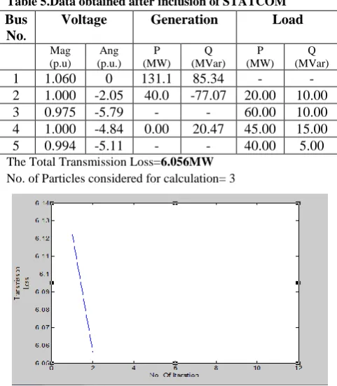
[image:3.595.303.544.105.151.2]

7. RESULTS AND GRAPH

Table 1. Demanded and generated power

Bus No. Demand Generated

P(MW) Q(MVar) P(MW)

1* 0 0 0

2 20 10 40

3 60 10 0

4 45 15 0

5 40 05 0

Table 2. Bus data

From Bus To Bus R(p.u.) X(p.u.) B(p.u)

1 2 0.02 0.06 0.06

1 4 0.08 0.24 0.24

2 4 0.06 0.18 0.18

2 3 0.04 0.12 0.12

2 5 0.06 0.18 0.18

4 5 0.01 0.03 0.03

4 3 0.08 0.24 0.24

Table 3.Data obtained from load flow analysis

Bus No.

Voltage Generation Load

Mag (p.u)

Ang (p.u.)

P (MW)

Q (MVar)

P (MW)

Q (MVar)

1 1.060 0 131.1 90.82 - -

2 1.000 -2.06 40.0 -61.59 20.00 10.00

3 0.972 -5.76 - - 60.00 10.00

4 0.987 -4.64 - - 45.00 15.00

5 0.984 -4.96 - - 40.00 5.00

The Total Transmission Loss=6.022 MW

Table 4.Transmission Losses for STATCOM on various Bus Locations

Bus Location Total Transmission Loss

3 6.140

4 6.056

5 6.073

From table 4, it is evident that it is not possible to locate the compensator randomly on the transmission n/w just by considering bus voltage.

Hence, we need an iterative method or an evolutionary algorithm for finding out the optimal bus location for locating a STATCOM.

7.1 Results for 5-bus n/w with STATCOM

Optimal Bus Location is bus 4.

[image:3.595.305.546.306.582.2]

The MVAr rating of STATCOM is 20.47 MVAr The Voltage Profile improved

.

Table 5.Data obtained after inclusion of STATCOM

Bus No.

Mag (p.u)

Ang (p.u.)

P (MW)

Q (MVar)

P (MW)

Q (MVar)

1 1.060 0 131.1 85.34 - -

2 1.000 -2.05 40.0 -77.07 20.00 10.00

3 0.975 -5.79 - - 60.00 10.00

4 1.000 -4.84 0.00 20.47 45.00 15.00

5 0.994 -5.11 - - 40.00 5.00

The Total Transmission Loss=6.056MW

No. of Particles considered for calculation= 3

Fig1. Graph obtained for PSO Algorithm Implementation

[image:3.595.44.286.441.745.2]

(4)

Fig2. Graph obtained for Bacterial Foraging Algorithm Implementation

No. of nodes taken in a set=1 No. of possible nodes =3

[image:4.595.304.549.323.473.2]

Fig3. Graph obtained for Plant Growth Algorithm Implementation

Table 6.9-bus Network Data

Bus No. Demand Generated

P(MW) Q(MVar) P(MW)

1* 0 0 0

2 0 0 163

3 0 0 85

4 0 0 0

5 90 30 0

6 0 0 0

7 100 35 0

8 0 0 0

9 125 50 0

Table 7.Branch data of 9-bus

From Bus To Bus R(p.u.) X(p.u.) B(p.u)

1 4 0.00 0.0576 0.00

4 5 0.017 0.092 0.158

5 6 0.039 0.17 0.358

3 6 0.00 0.0586 0.00

6 7 0.0119 0.1008 0.209

7 8 0.0085 0.072 0.149

8 2 0.00 0.0625 0.00

8 9 0.0032 0.161 0.306

[image:4.595.48.287.440.712.2]

9 4 0.001 0.085 0.176

Table 8.Data obtained from load flow analysis

Bus No.

Mag (p.u)

Ang (p.u.)

P (MW)

Q (MVar)

P (MW)

Q (MVar)

1 1.000 0 71.95 24.07 - -

2 1.000 9.67 163.0 14.46 - -

3 1.000 4.77 85.0 -3.65 - -

4 0.987 -2.41 - - - -

5 0.975 -4.02 - - 90.00 30.00

6 1.000 1.93 - - - -

7 0.986 0.62 - - 100.0 35.00

8 0.996 3.79 - - - -

9 0.958 -4.35 - - 125.0 50.00

The Total Transmission Loss=4.955MW

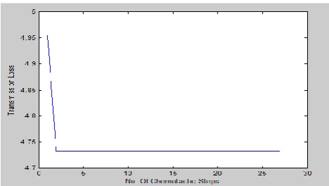
7.2 Results for 9-bus n/w with STATCOM

Optimal Bus Location is bus 9.

The MVAr rating of STATCOM is 46.67 MVAr . The Voltage Profile Improved.

Table 9.Data obtained with STATCOM

Bus No.

Mag (p.u)

Ang (p.u.)

P (MW)

Q (MVar)

P (MW)

Q (MVar)

1 1.000 0 71.95 24.07 - -

2 1.000 9.573 163.0 14.46 -

3 1.000 4.837 85.0 -3.65 - -

4 1.003 -2.36 - - - -

5 0.988 -3.90 - - 90.00 30.00

6 1.008 2.00 - - - -

7 0.994 0.67 - - 100.0 35.00

8 1.007 3.76 - - - -

9 1.000 -4.34 0.00 46.77 125.0 50.00 The Transmission Loss=4.733MW

(5)

7.3 Results for 30-bus n/w system

The network data was taken from [4].

[image:5.595.55.289.61.193.2]

The load flow output hasn‟t been included in this paper due to space constraints. However the overall voltage profile was found to improve on STATCOM inclusion, when compared to uncompensated system.

Table 10.Summarized data

System 30 bus

Optimal STATCOM Location

Bus 8

Optimal STATCOM Size 50.07 MVar

Transmission Loss of Uncompensated system

2.896MW

Transmission Loss of system with STATCOM

2.577MW

No. of Bacteria Considered= 5

8. CONCLUSION

With the above work we can find the optimal location and size of STATCOM to be used in a transmission network. With the above results it can be seen that STATCOM is a very suitable device for voltage profile improvement and on proper location it can also help in bringing down the transmission losses of the system, thus improving the overall efficiency of the network. The method suggested is quite simple and could be favorably used to find the most suitable location.

9. REFRENCES

[1] Narain G. Hingorani, Laszlo Gyugi, “Understanding Facts”, IEEE Power Engineering Society, Sponsor.

(6)

[3] R.K. Pancholi and K.S. Swarup, “Particle swarm optimization for security constrained economic dispatch,” in Proc. Int. Conf. Intelligent Sensing and Information Processing, 2004, pp. 7-12.

[4] J. Kennedy and R. Eberhart, “Particle swarm optimization,” in Proc. IEEE International Conference on Neural Networks, vol. 4, 1995, pp.1942-1948.

[5] Eberhart RC, Shi Y. Particle swarm optimization: developments, applications and resources. Proc Congr Evol Comput 2001;1:81–6.

[6] R.D. Zimmerman, C.E. Murillo-Sanchez, R. J. Thomas, “Matpower: Steady-State Operations, Planning and Analysis Tools for Power Systems Research and Education," Power Systems, IEEE Transactions on, vol. 26, no. 1, pp. 12, 19, Feb. 2011.

[7] E Acha, V.G. Agelidis, O Anaya-Lara, T J E Miller. “Power Electronic Control in Electrical Systems”. Chapter5

[8] R.C. Eberhart and Y. Shi, “Comparing inertia weights and constriction factors in particle swarm optimization,” in Proc. Congress on Evolutionary Computing, vol. 1, Jul. 2000, pp.84-88.

[9] W.J. Tang, Q.H. Wu and J.R. Saunders, "Bacterial Foraging Algorithm For Dynamic Environments," Evolutionary Computation. CEC 2006. IEEE Congress on, pp. 1324-1330, 2006.

[10]B.K. Panigrahi, V. Ravikumar Pandi, Renu Sharma, Swagatam Das, Sanjoy Das, “Multiobjective bacteria foraging algorithm for electrical load dispatch problem,” Energy Conversion and Management, 2011.Vol.52, pp. 1334–1342.

[11]Kim DH, Ajith Abraham, Cho JH. “A hybrid genetic algorithm and bacterial foraging approach for global optimization” Information Science 2007;177: 3918-37. [12]Wei Cai, Weiwei Yang and Xiaoqian Chen. “A Global

Optimization Algorithm Based on Plant Growth Theory:Plant Growth Optimization” International Conference on Intelligent Computation Technology and Automation, 2008.

[13]Wu Na, JIAO Yan-jun, Yu Jian-tao. “Fault Location of Distribution Network Based on Plant Growth Simulation Algorithm”. International Conference on High Voltage Engineering and Application, Chongqing,2008.

[14]Jing Ye, Fang Zong Wang. “A Refined Plant Growth Simulation Algorithm for Distribution Network Reconfiguration”. 978-1-4244-4738, IEEE 2009.

[15]Y. del Valle, Ronald G. Harley and G. K. Venayagamoorthy, “Comparison of Enhanced-PSO and Classical Optimization Methods: a case study for STATCOM placement”, IEEE Transactions, vol.5, no.1, pp.978, 5, September, 2009.

[16]Y. del Valle, J. C. Hernandez, G. K. Venayagamoorthy, “Optimal STATCOM Sizing and Placement Using Particle Swarm Optimization” , IEEE Transactions, vol.288, no.1, pp.4244, 3, June, 2006.

[17]Anant Baijal, Vikram Singh Chauhan, T.Jayabarathi, “Application of PSO, Artificial Bee Colony And Bacterial Foraging Optimization algorithms to Economic Load Dispatch: An Analysis”. IJCSI International Journal of Computer Science Issues, Vol. 8, Issue 4, No 1, July 2011.