Design and Implementation of a Noise Tolerant Polynomial Nonlinear ARX Model using the Averaging Wavelet Method

Design and Implementation of a Noise Tolerant

Polynomial Nonlinear ARX Model using the Averaging

Wavelet Method

Ehsan Khadem Olama

Ahwaz Petroleum University of Technology, Instrumentation & Automation

Department

Hooshang Jazayeri-Rad

Ahwaz Petroleum University of Technology, Instrumentation & Automation

Department

ABSTRACT

In this paper, a new nonlinear wavelet identification structure is proposed for high noise resistive soft sensors. This method uses proposedPolynomial Nonlinear Auto Regressive Exogenous Model, which can be solved with linear Gaussian Least Square Method, alongside the Averaging Wavelet Method (AWM) filter. AWM uses the approximation spaces for analyzing the signals and reduce the noise by a mean filtering over sub-resolutions. Conventional wavelet modeling methods use the detail spaces of the decomposed signal for signal modeling. Theapplication results show that this method can be more accuratein high level noisy environments than the conventional wavelet modeling methods cab tolerate.

General Terms

Wavelets, Nonlinear Auto Regressive Exogenous Modeling

Keywords

Averaging Wavelet Method, NARX, Noise tolerant modeling

1.

INTRODUCTION

The real world systems are rarely linear and well defined for controlling. Most systems show nonlinear behaviors. The low power μ-sensors produce low power results inPico-voltages or Pico-Amperes, which by transmitting over wires or wireless would be highly corrupted by noise. Employing these sensors to acquire data from nonlinear systems deteriorates the overall Signal to Noise Ratio (SNR). Analog hardware or digital hardware smoothing filters are conventionally employed to solve this problem. These kinds of filters reject the high frequencies or pass a frequency band that is needed in the process.

However, nonlinear systems may contain vital frequency components in the rejected region of the employed smoothing filters. These frequency components must be preserved to generate appropriate signals which will be used for system identification purposes. The solution is to develop an algorithm which trulyextracts the nonlinear system structures and parameters usingthe acquired unfiltered sensor signals. The developed algorithm achieves this goal by simultaneously denoising and identifying the system.

Studies on wavelet algorithms for denoising have recently been

frequencies in space bounds, which makes this technique different from conventional cut-off filters.

In section (2), Polynomial Nonlinear Auto Regressive Exogenous(PNARX) modeling will be introduced. Section (3) discussesthe Averaging Wavelet Method. In section (4) the ConventionalWavelet Method (CWM) for identification is studied.The newly proposed PNARX Averaging Wavelet Method (PNARX-AWM)has been discussed in section (5). In section (6),PNARX-AWM is compared to the conventional wavelet identification method.

2.

THE PNARX MODELING

For aSISO nonlinear system the general nonlinearmathematical

model can be given as:

 1 1

1 1

( ) , , , , , , , , ; ,

n n n n

n n n n

d y d y dy d u d u du

y t f u P W

dt dt dt dt dt dt

 

 

 

 _   _

 

(1)

According to Shannon sampling theory we can write this model as the following nonlinear difference equation [4]:







 

 







[ ] y k 1 , , y k p , u k 1 , u k 2 , , u[k r]; ,

y k f        P W (2)

𝑦is the output, 𝑢 is the input, 𝑘 is the sample index, 𝑃 is the parameters vector and 𝑊 is the uncertainty of the model. If we consider the effect of each shifted input and output individually, then the equation (2) can be separated as:

Figure 1.The PNARX identification method.

0 2 4 6 8 10 12 14 16 18 20

-1 -0.5 0 0.5

K

P

N

D

S

Training Real System Estimated System Absolet Error

0 2 4 6 8 10 12 14 16 18 20

-1 -0.5 0 0.5

K

In

p

u

t

We can find the Taylor series expansion of each function in equation (3) at its operating point as:

1 0 0 1 0 0 ( [ ]) ( [ ] ) ( [ ]) ( [ ] ) p r n n

iy n i

n n

n

iu n i

n

f y k i h y k i y

f u k i g u k i u

           





(4)

Equation (4) can be further simplified to:

2 11 12 13

1 2

1 22 23

1

1 2

12 13

[ ] [ 1] [ 1] ...

[ 1] [ 2] [ 2] ...

[ ] ...

[ 1] [ 1] ... [ ] [ ]

p p p p r r n n n pn n rn

y k a a y k a y k

a y k a y k a y k

a y k p

b u k b u k b u k r W k

                           (5)

This structure is nonlinear, however the equation is linear with respect to parameters which can be can be found by Gaussian Least Square method as:

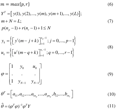
𝑚 = 𝑚𝑎𝑥 𝑝, 𝑟 (6)



(1), (2),..., ( ), ( 1),..., ( ) ;



;

( 1) ( 1) 1

T

p r

Y y y y m y m y L

m N L

p n r n N

         (7)









1 1 1 1

( ) ; 0,..., 1

( ) ; 0,..., 1

p r n i k _i n i k _i

y y m j k j p

u u m q k q r

       _   _    

 _   _   (8)

0 0

1 1

1

. . .

1 _{N N}

y u y y



             (9)

11, 12,..., 1p,..., p, 12,..., r

T

n pn rn

a a a a b b

 _{ } _{ (10)}

 1

( T ) T Y

_    ₍₁₁₎

Figure (1) demonstrates the input and output signals of a typical PNARX model. The upper figure shows the Polynomial Nonlinear Dynamic System (PNDS) of a 19 parameters system (in green), output of the identified system using the PNARX model (in dashed blue line) and the error between identified and the real system (in red). The figure shown at the bottom is the APRBS input to the system. The green portion of this figure is used for the training time and the blue portion is employed for testifying the system.

3.

AVERAGING WAVELET METHOD

(AWM)[5]

Here we use, the Haar wavelet transformexplained in[6]. A function 𝑓(𝑥) defined on [0,1] has an expansion in terms of Haar functions as follows:

Given any integer 𝐽 ≥ 0 in𝐿2 on [0,1] we have:

𝑓 𝑥 = 𝑓, ℎ𝑗 .𝑘 ℎ𝑗 .𝑘 𝑥 2𝑗₋₁

𝑘=0 ∞

𝑗 =𝐽

+ 𝑓, 𝑝𝐽 .𝑘 𝑝𝐽 .𝑘 𝑥 2𝑗₋₁

𝑘=0

(12)

In order to motivate a discrete version of this expansion, theDiscrete Haar Transform(DHT), we assume that we have only a finite, discrete approximation to 𝑓(𝑥). In this case, the most natural approximation is by the dyadic step function 𝑃𝑁𝑓(𝑥), where 𝑁 ∈ ℕ and 𝑁 > 𝐽. That is, given 𝑓(𝑥),

𝑓 𝑥 ≈ 𝑃_𝑁𝑓 𝑥 = 𝑓, 𝑃_𝑁,𝑘 𝑃_𝑁,𝑘(𝑥)

2𝑁₋₁

𝑘=0

(13)

Thus, the Haar coefficients of 𝑓(𝑥) can be approximated by the Haar coefficients of𝑃𝑁𝑓(𝑥). That is:

𝑓, ℎ𝑗 ,𝑘 ≈ 𝑃𝑁𝑓, ℎ𝑗 ,𝑘 𝑎𝑛𝑑 𝑓, 𝑝𝑗 ,𝑘 ≈ 𝑃𝑁𝑓, 𝑝𝑗 ,𝑘 (14) Therefore, we can make the following definition:

Given 𝐽, 𝑁 ∈ ℕ with 𝐽 < 𝑁 and a finite sequence𝑐0=

𝑐0(𝑘) 2

𝑁₋₁

𝑘=0, the DHT of𝑐0 is defined by:

𝑑𝑗 𝑘 : 1 ≤ 𝑗 ≤ 𝐽; 0 ≤ 𝑘 ≤ 2𝑁−𝑗− 1

∪ 𝑐𝐽 𝑘 : 0 ≤ 𝑘 ≤ 2𝑁−𝐽− 1 (15)

, where:

𝑐𝑗 𝑘 =

1

2𝑐𝑗 −1 2𝑘 + 1

2𝑐𝑗 −1 2𝑘 + 1 (16)

𝑑𝑗 𝑘 =

1

2𝑐𝑗 −1 2𝑘 − 1

2𝑐𝑗 −1 2𝑘 + 1 (17)

The inverse DHT is given by the formula:

𝑐𝑗 −1 2𝑘 =

1 2𝑐𝑗 𝑘 +

1

2𝑑𝑗(𝑘) (18)

𝑐𝑗 −1 2𝑘 + 1 =

1 2𝑐𝑗 𝑘 −

1

2𝑑𝑗(𝑘) (19)

Based on the Haar transform the AWM is constructed. The traditional wavelet denoising method is based on computing the two composed and detail vectors of signal, then thresholding details in each𝑑𝑗 and consequently reconstructing the signal𝑐𝑗 +1. However,the detail vectors are important and the noise is unwanted. We use the DHT’s equation(16) and the detail vectors are ignored. From equation (16) we find the composition vectors

for 𝐿 ≤ 𝑁/2. Then we write the𝑆𝑖 sequences using𝑐𝑖 as:

𝑆𝑖 𝑘 =

𝑐𝑖 ₂𝑘𝑖

2𝑖 ; 1 ≤ 𝑖 ≤ 𝐿; 0 ≤ 𝑘 ≤ 2

𝑁_{− 1} (20)

[image:2.612.53.283.291.506.2]

𝑆 𝑘 = 𝑆𝑖 𝑘

𝐿 𝑖=1

𝐿 (21)

Then we can repeat this procedure 𝑅 times. Each time 𝑆(𝑘) is used as input to the algorithm. The codes and results can be downloaded from[4].

4.

OFFLINE

PNARX

USING

THE

CONVENTIONAL WAVELET METHOD

(PNARX-CWM)

For illustration, consider the nonlinear system shown in figure (2). The output of the system is the summation of two

exponential functions of input signal (with coefficient constants of 1 and 2) as:

𝑦 𝑡 = 𝑒𝑢(𝑡)_{+ 𝑒}2𝑢(𝑡) (22)

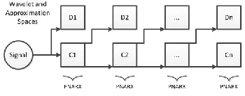
The structure of the PNARX-CWM can be seen in figure (3). Each wavelet space and the last approximation space havetheir own PNARX model.

Figure (4) shows the Amplitude-modulated Pseudo Random Binary Signal (APRBS)described in [7].In this work, this signal is used as the excitation signal.Thelength, amplitude and sampling time of the excitation signal must be chosen to capture the nonlinearity and frequency range of the system to be identified.

As shown in figure (4), after identification of the system, the identified parameters have been testified by a variable frequency non-stationary input and the simulation results are shown in figure (6):

0.5cos(2 ) 1 6 8 ( ) 0.5cos(4 ) 1 8 10 0.5cos(8 ) 1 10 12

t t

u t t t

t t

 

 

 

  

 

_   

 _{  }



(23)

By adding noise to the signal from 1% to 100%,as shown in table (1), the MSE obtainedusingPNARX-CWMwill be around 43 to 68. As shown in this table the identification technique deteriorates the MSE if the level of added noise is less than 50%. Improvement in the magnitudes of MSE is achieved for the level of noise greater than 50%. At 100% noise level, the MSE of the identified signal will almost be half of the MSE of the original signal. According to table (2), the SNR of this method will vary from 4 to 6.

5.

OFFLINE

PNARX

USING

THE

AVERAGING

WAVELET

METHOD

(PNARX-AWM)

Unlike PNARX-CWM, this method identifies each approximation space in lower resolutions and reconstructs the

original signal by the AWM algorithmexplained in section (3). The structure of the identification algorithm is shown in figure (5) and the simulation results are shown in figure (7).

[image:3.612.56.259.205.299.2]

For identification, we use an APRBS signal in offline mode and then testify the identified system by non-stationary input given by equation (26). As shown in table (1) the identification technique deteriorates the MSE if the level of added noise is less than 20%. Reduction in the magnitudes of MSE is achieved for the level of noise greater than 20%. At 100% noise level, the MSE of the identified signal will almost be one tenth of the MSE of the original signal. Therefore, the level of achieved MSE for this technique is always less than the MSE obtained in PNARX-CWM. According to table (2), the SNR of this method will vary from 10 to 13, which are always better than the SNR quoted for PNARX-CWM.

[image:3.612.340.551.244.339.2]

Figure 2.Nonlinear system in the presence of noise.

Figure 3. Each wavelet space and the last approximation space have its own PNARX identification.

Figure 4. The APRBS excitation signal (the upper signal). The variable frequency signal (the lower signal) used for testifying the identified model.

18 20 22 24 26 28 30 32 34 36 38

-1 -0.5 0 0.5 1

t[s]

E

xci

ta

ti

o

n

S

ig

n

a

l

18 20 22 24 26 28 30 32 34 36 38

0.5 1 1.5

t[s]

T

e

stifyin

g

S

ig

n

a

l

[image:3.612.353.528.432.501.2]

6.

CONCLUSIONS

The results in table (1) and table (2) show that the developed PNARX-AWM method outperforms the conventional wavelet identification method for signals withhigh level of noises. The proposed method results a substantial reduction of MSE. In addition, a significant improvement in SNR is achieved. These

data are derived using the PNARX and Wavelet structure with the following parameters: N=12, v=6, p=5, r=1, np=3, nr=2.Codes and results of simulation can be downloaded from: http://ekoshv.persiangig.com/MATLABCODES/PNARX_ACW M/PNARXACWM.rar

7.

REFERENCES

[1] Radunovic, D. P., 2009, "Wavelets from Math to Practice," Springer, Berlin.

[2] Aadaleesan, P., and Saha, P., 2008, "Nonlinear System Identification Using Laguerre Wavelet Models," Chemical Product and Process Modeling, 3(2).

[3] Ebadat, A., Noroozi, N., Safavi, A. A., and Mousavi, S. H., 2010, "Modeling and control of nonlinear systems using novel fuzzy wavelet networks: The modeling approach " Decision and Control (CDC2010) IEEE, Atlanta, GA. [4] Olama, E. K., 2011, "Averaging Wavelet Method:

MATLAB codes,"

http://ekoshv.persiangig.com/MATLABCODES/AWM/AW M.zip.

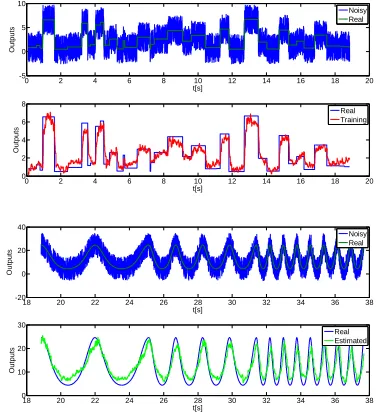
Figure 6. Identification of the nonlinear system using PNARX-CWM (the training is performed using 50% input-output noisy data).

0 2 4 6 8 10 12 14 16 18 20

-5 0 5 10 15 t[s] N o n lin e a r S yste m Noisy Real

0 2 4 6 8 10 12 14 16 18 20

-5 0 5 10 t[s] N o n lin e a r S yste m Training Real

18 20 22 24 26 28 30 32 34 36 38

-20 0 20 40 t[s] N o n lin e a r S yste m Noisy Real

18 20 22 24 26 28 30 32 34 36 38

-10 0 10 20 30 t[s] N o n lin e a r S yste m Estiimated Real

Table 1.MSE comparison of PNARX-CWM and PNARX-AWM. Noise Percent Noisy System MSE MSE of PNARX-CWM MSE of PNARX-AWM

1% 0.013 68.71 8.161

5% 0.339 51.79 7.665

10% 1.388 50.37 9.189

20% 5.440 58.65 10.27

50% 33.80 53.65 10.86

80% 86.75 43.83 12.65

100% 138.3 63.17 14.17

Figure 7. Identification of the nonlinear system using PNARX-AWM (the training is performed using 50% input-output noisy data).

0 2 4 6 8 10 12 14 16 18 20

-5 0 5 10 t[s] O u tp u ts Noisy Real

0 2 4 6 8 10 12 14 16 18 20

0 2 4 6 8 t[s] O u tp u ts Real Training

18 20 22 24 26 28 30 32 34 36 38

-20 0 20 40 t[s] O u tp u ts Noisy Real

18 20 22 24 26 28 30 32 34 36 38

0 10 20 30 t[s] O u tp u ts Real Estimated

Table 2.SNR comparison of CWM and PNARX-AWM. Noise Percent Noisy System SNR SNR of PNARX-CWM SNR of PNARX-AWM

1% 41.62 4.61 13.11

5% 27.71 5.161 13.44

10% 21.61 4.599 12.49

20% 15.73 4.427 12.55

50% 8.352 6.299 11.84

80% 5.205 5.693 11.91

[image:4.612.59.266.83.298.2] [image:4.612.327.553.113.261.2] [image:4.612.77.270.352.559.2]

[5] E.K. Olama, and Valiloo, S., 2011, "A fast wavelet denoising method," Computer Research and Development (ICCRD)Shanghai pp. 492 - 494.

[6] F.Walnut, D., 2002, An Introduction to Wavelet Analysis, Birkhauster.