Blast Waves in Multi Component Medium with Thermal Relaxation

http://dx.doi.org/10.4236/ns.2014.612096

Blast Waves in Multi-Component Medium

with Thermal Relaxation

Vyacheslav O. Vakhnenko

Institute of Geophysics, National Academy of Sciences of Ukraine, Kyïv, Ukraine Email: [email protected]

Received 26 June 2014; revised 30 July 2014; accepted 12 August 2014

Copyright © 2014 by author and Scientific Research Publishing Inc.

This work is licensed under the Creative Commons Attribution International License (CC BY). http://creativecommons.org/licenses/by/4.0/

Abstract

hy-drodynamics it is possible to explain the observed phenomena and estimate the efficiency of me-dium as localizer of the shock wave action.

Keywords

Structured Medium, Asymptotic Model, Relaxation, Nonlinear Wave, Explosion

1. Introduction

Natural media are not structureless. The experiments have shown that the intrinsic structure of a medium influences the wave motions [1]-[7]. Existing inhomogeneities complicate the problem and, at the same time, are fully manifested under the propagation of nonlinear waves.

The wave processes in heterogeneous media are usually described in terms of more or less complicated mod- els. Under the conditions of local equilibrium, the media are traditionally modeled irrespective of their structure. In the framework of continuum mechanics, the known idealization of a real medium as a homogeneous one has been fairly successive in the description of wave processes (see, for instance, [8]-[10]). The continuum models are commonly applied to the mixtures whose dispersive dissipative properties are treated with regard for the in- teractions between the components [11]-[15]. On this level the media are modeled in the framework of a homo- geneous elastic, viscous elastic, and elastic plastic medium [12] [16]. In this case the features of the structure in medium are taken into account indirectly through the kinetic parameters (relaxation time, viscous coefficients etc.) [3] [4] [9] [11]-[16].

The model of multivelocity interpenetratable continua was developed in terms of classical continuum mechanics [17] and statistical physics [18] in order to describe the dynamical behavior of multi-component media. A fundamental assumption in the theory of mixtures [15] reproduces the assumption in the model of multivelocity interpenetratable continua [17]; namely that each micro-volume dv is occupied by a particle of each constituent. The equations of motion for each component involve the terms describing the mass, force and energy interactions between the components. The problem is complicated by the necessity to employ, in the general case, the experimental data for establishing theoretical relations between the macroparameters at the component interaction level. Moreover, if the component interaction is determined, these models would be indispensable in the theory of multi-component media.

In all the models mentioned, the formalism of continuum mechanics is based on the principle of local action as well as on the generalization of the mechanics laws relating the point mass to the continuum [10].

When going from the integral equations to differential balance equations, the existence of a differentially small microvolume dv is assumed. On the one hand, this volume is so small that the mechanics laws of the point can be extended to the whole microvolume. On the other hand, the volume contains so many structural elements of the medium that, in this sense, it can be regarded as macroscopic one in spite of its smallness as compared to the entire volume occupied by the medium. So, the passage to the differential balance equations is based on the assumption that microstructural scales ε are small as compared to the characteristic macroscopic scale of the

λ

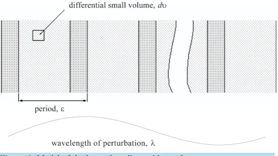
, and the passage should be made to the limiting case ε λ →0. Contraction of the volume dv to the point in the general case is correct for continuous functions [10] [15]. This means that all points within the differentially small volume are equivalent. Hence, for the case of a mixture, the equivalence of the points implies that field characteristics should be averaged over dv. Hence, it is assumed that the equations of motion can be written in terms of average density, mass velocity, and pressure of each individual component. We note that these models do not contain explicit sizes of components.

[image:3.595.157.442.85.245.2]

Figure 1. Model of the layered medium with two homogeneous components in period.

We describe the wave processes in non-equilibrium heterogeneous media in terms of an asymptotic averaged model [19]-[23]. In this case the obtained integral differential system of equations cannot be reduced to the average terms (pressure, mass velocity, specific volume) and contains the terms with characteristic sizes of individual components.

On the microstructure level of the medium, the dynamical behavior is governed only by the laws of thermo- dynamics. On the macrolevel, the motion of the medium can be described by the wave-dynamical laws for the averaged variables with the integrodifferential equation of state containing the characteristics of the medium microstructure. A rigorous mathematical proof is given to show that on the acoustic level, the propagation of long waves can be properly described only in terms of dispersive dissipative properties of the medium, and in this case, the dynamical behavior of the medium can be modeled by a homogeneous relaxing medium. However, finite-amplitude long waves respond to the structure of the medium in such a way that the homogeneous me- dium model is insufficient for the description of the behavior of the structured medium. An important result that follows from this model is that, for a finite-amplitude wave, the structure of medium (in particular, existence of microcracks) produces nonlinear effects even if the individual components of the medium are described by a li- near law.

We have considered averaged systems of hydrodynamical equations in both Lagrangian and Eulerian coordi- nates. These systems are not expressed in the average hydrodynamical terms; hence the dynamical behavior of the medium cannot be modeled by a homogeneous medium even for long waves, if they are nonlinear. The structure of the medium influences the nonlinear wave propagation. The heterogeneity of the structure of me- dium always introduces additional nonlinearity that does not arise in a homogeneous medium.

We suggest a transformation that enables one to reduce, with certain accuracy (the transformation is exact for planar symmetry as well as for stationary flows), the known solutions of gas-dynamic problems to the two-phase media with arbitrary volume portion of incompressible components.

This transformation enables one to obtain the solution of many problems for multi-component media with in-compressible phases from the similar problem for perfect gas. In this case it is not necessary to solve directly the problem for the medium with incompressible component, and it is sufficient just to transform the known solu-tion of the similar problem for a homogeneous medium. Thus, the solusolu-tions of many hydrodynamical problems for multi-component media with incompressible phases can be obtained without solving the initial system of equations. The scope for the suggested transformation is demonstrated by the reference to the strong explosion state in a two-phase medium.

on the thermal relaxation time in order to provide a deeper understanding of the damping of shock waves in such media and to determine their effectiveness as localizing media. Besides, it is of interest to define the dependence of shock wave attenuation on the shock loading, especially on the explosion energy.

2. Asymptotic Averaged Model for Structured Medium

The current status of experimental researches demands to develop the models of dynamical behavior of media with account of their inner structure. The real media are not structureless. For example, the geophysical medium has a complicated hierarchical structure. It turns out that the ratio of typical sizes between the neighboring hierarchical levels is a constant value [5] [6]. The inner structure of a medium affects the propagation of waves. Fast high-gradient processes, such as earthquakes, explosions, etc., lead to irreversible processes [6] [7].

Within continuum mechanics [24] the known idealization of a real medium as homogeneous has a wide application to model their dynamic behavior. Traditionally, it was considered that in heterogeneous media with wavelength appreciably exceeding the size of the structural heterogeneities, the perturbations propagate in the same way as in homogeneous media [8] [9] [15]. However, this statement should be proved, and we shall show that this approximation is not universally true.

The properties of a medium deviate from the equilibrium state under the propagation of intensive waves. Moreover, an unperturbed medium can be in one of unstable stationary states. So, a geophysical medium, within a current physical concept, is an open thermodynamic system, which essentially influences on the exchanges of energy and mass. Thus, a description of open systems should take into account the peculiarities of their inner structure, dynamical processes occurring on the level of structural elements. What is more, the state of media under the action of high-frequency wave perturbations departs from equilibrium, and, thus, the behavior of media can not be described in the framework of equilibrium thermodynamics. Consequently, there is necessity to develop the new mathematical models in order to take into account the nonlinear wave perturbations and irreversible inner exchange processes.

2.1. Background and Initial Equations

The simplest heterogeneous media for which the effect of the structure can be analyzed are media with a regular structure. Features of the propagation of long wave perturbations will be investigated by using as an example, a periodic medium under conditions of an equality of stresses and mass velocities on the boundaries of neighboring components. It is supposed that the microstructure elements of medium dv (see Figure 1) are large enough that it is possible to submit to the laws of classical continuum mechanics for each individual component. At the same time the inner processes in each component will be considered within a relaxation approach. The notions based on the relaxation nature of a phenomenon are regarded to be promising and fruitful. We consider that the properties of the medium, such as density, sound velocity and relaxation time vary in a periodic manner (although this assumption is unessential in the final result).

2.1.1. Motion Equations for Individual Component

The analysis of wave motions is based on the hydrodynamic approach. This restriction can be imposed for the modeling of nonlinear waves in watersaturated soils, bubble media, aerosols, etc. [12] [13]. The set of acceptable media could be extended to solid media where the powerful loads are studied in the condition that the strength and plasticity of the material can be neglected [25]. In the hydrodynamic approach we have considered the media without tangential stresses while there are equalities of the stresses as well as of mass velocities on boundaries of neighboring components. Also, we assume that the medium is barothropic. The individual compo- nents of the medium are considered to be described by the classical equations of hydrodynamics. In the Lagrangian coordinate system

( )

l t, the equations of one-dimensional motion for each individual component have the form

0 1

0

, ,

0.

r V r

u

V t

l

u r p

V

t l l

ν ν

ν −

∂ ∂

= =

∂ ∂

∂ ₊   ∂ ₌

 

∂   ∂

The equation of continuity can also be used in the alternative form

1

0 0.

V r u

V

t l

ν ν

ν −

∂ ₋ ∂ ₌

∂ ∂ (2.1.2)

Here _{V =}ρ−1

is the specific volume, ν is a parameter of symmetry, where

ν

=1 is planar symmetry, 2

ν

= is cylindrical one,

ν

=3 is spherical one; the index 0 relates to the initial state. The other notations are those that are generally accepted.

Conditions for matching are the equality of mass velocities and pressures on the boundaries of the components

[ ]

u =0,

[ ]

p =0. (2.1.3)

2.1.2. Dynamic State Eqution

Considering the models of a relaxing medium as more general than the equilibrium models for describing the evolution of high-gradient waves, we will take into account the relaxing processes for each component. Thermodynamic equilibrium is disturbed owing to the propagation of fast perturbations in a medium. There are processes of the interaction that tend to return the equilibrium. The parameters characterizing this interaction are referred to as the inner variables unlike the macroparameters such as the pressure p, mass velocity u, and density

ρ

. In essence, the change of macroparameters caused by the changes of inner parameters is a relaxation process. From the nonequilibrium thermodynamics standpoint, the models of a relaxing medium are more general than the equilibrium models for describing the wave propagation.

An equilibrium state equation of a barothropic medium is an one-parameter equation. As a result of relaxation, an additional variable ξ (inner parameter) appears in the state equation. It defines the completeness of the relaxation process

(

,

)

.

p= p ρ ξ (2.1.4)

There are two limiting cases:

(i) the lack of the relaxation (inner interaction processes are frozen) ξ =1,

( )

,1 _f

( )

,

p= p ρ = p ρ (2.1.5)

(ii) the relaxation complete (there is the local thermodynamic equilibrium) ξ =0,

(

, 0

)

_e

( )

.

p= p ρ = p ρ (2.1.6)

The state Equations (2.1.5) and (2.1.6) are considered to be known. These relationships enable us to introduce the sound velocities for fast processes

2

d d

f f

c = p ρ (2.1.7)

and for slow processes

2

d d .

e e

c = p ρ (2.1.8)

The slow and fast processes are compared by means of the relaxation time τp. The dynamic state equation is

written down in the form of the differential first-order equation

(

)

2

d d

0.

d d

p f e

p c

t t

ρ

τ  ₋ − ₊ ρ ρ_{− =}

 

  (2.1.9)

The equilibrium equations of state are considered to be known

0

2

0 d .

p

e e

p c p

ρ ₋ρ ₌ −

∫

(2.110)

Clearly, for the fast processes

(

ωτ_p1

)

we have the relation (2.1.5), and for the slow ones

(

ωτ_p1

)

we obtain (6).

and Leontovich [29] (see also Section 81 in [24]). We note that the mechanisms of the exchange processes are not defined concretely when deriving Equation (2.1.9), and the thermodynamic and kinetic parameters appear only in this equation. These characteristics can be found experimentally.

The phenomenological approach for describing the relaxation processes in hydrodynamics has been developed in many publications [12] [13] [24] [27]. The dynamic equation of state was used (a) for describing the propagation of sound waves in a relaxing medium [24], (b) for taking into account the exchange processes within media (gas-solid particles) [27], (c) for studying wave fields in gas-liquid media [12] and in soil [13]. In most works, the equation of state has been derived from the concept of concrete mechanism for the inner process. Within the context of mixture theory, Biot [11] attempted to account for the non-equilibrium in velocities between components directly in the equations of motion in the form of dissipative terms.

We assume that the relaxation time and sound velocities do not depend on time, but they are functions of pressure and the individual properties of the components. This means that in the process of a relaxation interaction we can take into account the exchange of moment and heat but not that of mass. Peculiarities of the intrastructure interaction are determined by the dynamic equation of state for each component.

The equations of motion (2.1.1) have been written in the Lagrangian coordinate system. The necessity of such a description stems from the fact that the dynamic equation of state (2.1.9) has been written to the mass element of a medium. Besides, the use of the Lagrangian coordinates is important for the application of the method of asymptotic averaging, since in these coordinates the structure is independent of a wave process.

2.2. Asymptotic Averaged System of Equations

A regularity of structure and a nonlinearity of long-wave processes investigated here specify the choice of mathematical methods. One way of studying this heterogeneous medium is based on a method of asymptotic averaging of equations with high-oscillating coefficients [30]-[33]. The essence of this method consists in the application of a multiscale method in combination with space averaging. In accordance with this method, the mass space coordinate m l V0

ν

= is divided into two independent coordinates: slow coordinate s and fast one

ξ, wherein

1

, .

m s

m s

εξ ε

ξ

−

∂ ∂ ∂

= + = +

∂ ∂ ∂ (2.2.1)

The slow coordinate s corresponds to a global change of the wave field and s is a constant value during a period, while the fast coordinate ξ traces the variations of a field in the structure period. The dependent functions are presented as a degree series over the structure period ε

( )

( )

₍

₎

( )

₍

₎

( )

₍

₎

( )

( )

₍

₎

( ) ( )

₍

₎

( )

( )

₍

₎

( )

₍

₎

( )

₍

₎

( )

( )

( )

(

)

( )

( )

(

)

( )

( )

(

)

0 1 2 2

0 1 2 2

0 1 2 2

0 1 ₂ 2

, , , , , , ,

, , , ( , , ) , ,

, , , , , , ,

, , , , , , ,

V m t V s t V s t V s t

p m t p s t p s t p s t

u m t u s t u s t u s t

rν m t rν s t rν s t rν s t

ξ ε ξ ε ξ

ξ ε ξ ε ξ

ξ ε ξ ε ξ

ξ ε ξ ε ξ

= + + +

= + + +

= + + +

= + + +

  



(2.2.2)

where p( )i , u( )i , V( )i , r( )i are defined as the one-period functions of ξ. In the Lagrangian mass coordinates the period is a constant which allows the averaging procedure to be performed.

We now will prove that p( )0 = p( )0

( )

s t, , p( )1 = p( )1

( )

s t, , u( )0 =u( )0

( )

s t, ,

( )

rν ( )0 =

( )

rν ( )0

( )

s t, are inde- pendent of the fast variable ξ. Indeed, after substitution of Equations (2.2.1) and (2.2.2) into the initial equations of motion, we obtain

( )

( )

( )

( )

( )

( ) ( )

0 0 1

0

1 0

0,

r r r

V s

ν ν ν

ε ε

ξ ξ

−

 

∂ _∂ ∂ _

− + _ − − _+ =

∂ _ ∂ ∂ _

 



( )0 ( )0 0

0, r

u t

ε _ −∂ _+ =

∂

( )

( ) ( ) ( )

_{( )}

( ) ( )

( )

( ) ( )

_{( )}

( ) ( )

0 0 0

0 0

1 1 0 1

0 1

1 0

1 1

(

0,

p u p

r r t s p p r r ν ν ν ν

ε ν ε ν

ξ ν ν ξ ξ − − − − −  ∂ ∂ ∂ − + _ + ∂ _ ∂ ∂  ∂ ∂ + + _+ = ∂ _{∂ } 

( )

₁ ( ) ( )0 _{0 ( )}

_{( )}

₁ ( ) ( )0 ₀

_{( )}

₁ ( ) ( )1 ₀

_{( )}

₁ ( ) ( )0 ₁

0

1 0

0,

r u _V r u r u r u

t s

ν ν ν ν

ε ν ε ν ν ν

ξ ξ ξ

− − − − −   ∂ _∂ ∂ ∂ ∂ _ − + _ + − − _+ = ∂ _ ∂ ∂ ∂ ∂ _   

According to the general theory of the asymptotic method, the terms of equal powers of ε should vanish

independently of each other. Thus, ∂p( )0 ∂ =ξ 0, ∂u( )0 ∂ =ξ 0, _∂

( )

_rν−1 ( )0 _{∂ =}ξ ₀

, i.e. p( )0 = p( )0

( )

s t, ,

( )0 ( )0

_{( )}

,

u =u s t , r( )0 =r( )0

( )

s t, are independent of ξ. Furthermore

( )

( )

( )

( ) ( ) ( ) ( ) ( )

( )

( ) ( )

( )

( ) ( ) ( )

( )

( ) ( )

( )

( ) ( )

( )

( ) ( ) 0 1 0 0 0

0 0 1

0 0

1 1

0 ₀ 1 ₀ 0 ₁

1 1 1

0 , , 0, 0. r r V s r u t

u p p

r r

t s

r u r u r u

V

t s

ν ν

ν ν

ν ν ν

ξ

ν ν

ξ

ν ν ν

ξ ξ − − − − − ∂ ∂ + = ∂ ∂ ∂ = ∂ ∂ ∂ ∂ + + = ∂ ∂ ∂ ∂ ∂ ∂ ∂ _{− − − =} ∂ ∂ ∂ ∂ (2.2.3)

Thus, we can average the equations during the period ξ. We define 1

( )

0 dξ

⋅ =

_∫

⋅ , and perform the normali-

zation 1 0dξ =1

∫

. Since p( )1 , ( )1

u and r( )1 are periodic, the integrals can be calculated as ( )1

0

p ξ

∂ ∂ = ,

( )1

0

u ξ

∂ ∂ = , ∂r( )1 ∂ξ =0. Moreover, as u( )0 =u( )0 p( )0 = p( )0 , than ∂p( )1 ∂ =ξ 0. This means that ( )1

p does not also depend on ξ. After integrating over the structure period the equations containing the value of zero order of ε, we obtain the averaged system

( )

( ) ( ) ( ) ( ) ( )

( )

( ) ( ) ( )

_{( )}

( ) ( ) 0 0 0 0 0 0 0 1 0

0 1 0

, , 0, 0 r V s r u t u p r t s

V r u

t s ν ν ν ν ν − − ∂ = ∂ ∂ = ∂ ∂ ∂ + = ∂ ∂ ∂ ∂ − = ∂ ∂ (2.2.4)

with the averaged equation of state

( ) ( )

( )

( ) ( )

( )

(

( )

( )

( )

)

2 0 0

0 0 0

2 0

d d _e d .

f _{p e}

V _V

V p V V p t

c τ _{V p}

= − − − (2.2.5)

Choosing the wavelength

λ

to be large enough we can always reduce the effect to zero from other approximation terms.

The averaged system of Equations (2.2.4), (2.2.5) is an integro-differential one and, in the general case, is not reduced to the averaged variables p, u and V( )0 . The derivation of Equations (2.2.4), (2.2.5) relates to a rigorous periodic medium. However, it may be shown that Equations (2.2.4), (2.2.5) are also relevant to media with a quasi-periodic structure. Indeed, the pressure p and the mass velocity u are independent of the fast variable ξ. Hence on a microscale ξ, the action is statically uniform (waveless) over the whole period of the medium structure, while on the slow scale s, the action of perturbation is manifested by the wave motion of the medium. On a microlevel the behavior of medium adheres only to the thermodynamic laws. There is a mechanical equilibrium. On a macrolevel, the motion of medium is described by the wave dynamics laws for averaged variables. Mathematically, in the zero-order case of ε, the size of the period is infinitesimal

(

ε →0

)

. This signifies that the location of particular components in the period is irrelevant. The Equations (2.2.4), (2.2.5) do not change their form if the components are broken and/or change their location in an elementary cell. This means that Equations (2.2.4), (2.2.5) describe the motion of any quasi-periodic (statistical heterogeneous) medium which has a constant mass content of components on the microlevel, and the location of these components within the cell is not important.

In the case of nonlinear wave propagation, the individual components suffer different compressions. The structure of medium is changed, with the result that the averaged specific volume V is changed. This change differs from the change of the specific volume for homogeneous medium under the same loading. Thus, the structure of medium is manifested in the wave motion, despite the fact that the equations of motion (2.2.4) (but not the equation of state) are written down for the averaged values u, p, V only.

2.3. System of Equations in Eulerian Coordinates

In certain cases of theoretical analysis it is more convenient to use the Eulerian coordinate system. The immediate employment of the averaging asymptotic method in Eulerian variables is impossible because of the variability of the microstructure sizes. However, from the zero approximation in the equations of motion (2.2.1), which are presented by the averaged values p, u, V , the equations can be rewritten in the Eulerian system of coordinates

(

r t,E

)

by means of a transformation from the Lagrangian system

( )

s t, [19]-[23]

( )

, , _E .

r=r s t t =t (2.3.1)

There is an important presumption that the velocity of the particle in the zero approximation is constant over a period of the structure and, consequently, we can describe an averaged trajectory for the particle

( )

,

_{( )}

, . s

r s t

u s t t

∂

 

=

 _∂ 

  (2.3.2)

From the physical point of view, it is clear that the position of the particle is unambiguously defined by its coordinate and time

1

drν =A sd +νrν−u td , t_E =t. (2.3.3) From the mathematical point of view this means that in the transformation (2.3.3) the value drν is a total differential. Therefore, we must have

1

.

A r u

t s

ν

ν −

∂ ₌∂

∂ ∂

This condition is satisfied if A= V , because the equation converts into the continuity Equation (2.2.4). We obtain the following transformation between Lagrangian and Eulerian systems of coordinates:

1

dr V ds r u td , tE t.

ν _{= +ν} ν− ₌

(2.3.4)

It is reasonable to define the slow Lagrangian coordinate (non-mass one) as

.

Equations (2.2.4) in the Eulerian system of coordinates then take the form

1 1 1

0,

0. E

E

V r u V

t r

u u p

u V

t r r

ν − − −

∂ ∂

+ =

∂ ∂

∂ ₊ ∂ ₊ ∂ ₌

∂ ∂ ∂

(2.3.6)

It is convenient to determine the fast Eulerian coordinate ζ as

( )

.

t

ζ ρ

ξ ρ ξ

∂  ₌

_∂ 

 



(2.3.7)

It should be noted that the average density ρ in the Eulerian coordinates is a value usually used for density. A chain of identities

( )

1 1

1

0 0

d d

V V ξ ξ V ρ ζ ρ

ρ −

=

_∫

=

_∫

= 

 (2.3.8)

proves that V −1 is the average density of the medium in the Eulerian coordinates. Note that ρ≠ ρ . The value ρ is a real density. The value V is the specific volume averaged in units of mass over the period and

it is expressed as the ratio of the volume to the mass inside this volume. This value can be determined experimentally. At the same time the averaged values p and u coincide in both Lagrangian and Eulerian systems of coordinates. Now the equations of motion (2.3.6) can be written in the usual form of the averaged density ρ.

We have proved in Ref. [19] that the known Lyakhov model for the natural multi-component media [13] is an actual case of the asymptotic averaged model, i.e., it is inherently asymptotic.

2.4. Analysis of the Averaged System of Equations

Now we will study some general properties of the averaged system of equations, and will obtain a rigorous mathematical proof that for the acoustic level the long wave dynamic behavior of the medium with a microstructure can be modeled within the framework of a homogeneous relaxing medium. At the same time the description of nonlinear waves can not be reduced to the average characteristics of wave field.

2.4.1. Acoustic Waves

Let us consider an acoustic wave

(

p′= −p p0,p′ p0

)

. We shall prove that the propagation of the acoustic waves in a periodic medium with a calculable number of relaxation components is similar to that in a homogeneous medium with the same number of independent relaxation processes.

Now we shall show it for a two-layer periodic medium with one process of relaxation in each structure element. The averaged equation of state (2.2.5)

( )

(

( )

)

2

2

d d e d

e f

V V

V p V V p t

V p

c τ

= − − −

for small perturbations in this medium can be represented as

(

)

₍

₎

(

)

(

)

2 2 2 2 2 2

1 1 1 2 2 2

2 2

1per 2 per

2 2 2 2 2

1 1 2 2

1 ,

d d

1 1

d d

1 ,

e f e f

f

e e e

V c c V c c

V V c p p p

t t

V c V c V c

τ τ

− ₋ − − ₋ −

′ ′ ′ ′

− = + + −

+ +

= + −

 

 

(2.4.1)

For comparison we take the homogeneous medium with two independent relaxation processes. The state equation of this medium for small perturbations has a form [24]

(

)

(

)

2 2 2 2 2 2

1 1 2 2

2 2

1hom 2 hom

2 2

,

d d

1 1

d d

.

e f e f

f

f fi i

V c c V c c

V V c p p p

t t

c c

τ τ

− − − −

− −

− −

′ ′ ′ ′

− = + +

+ +

=

∑

(2.4.2)

It should be noted that the alphanumeric indices for the homogeneous medium and for the periodic one have a reverse succession. Here, index 1 relates to the first relaxation process, and index 2—to the second process.

Now we can write six relationships

(

)

(

)

(

)

2 2 2 2 2 2

per hom

2 2 2 2 2 2 2 2

hom

per hom 1 2

,

, ,

, , 1 , 1, 2.

i i ie if ei fi

e ei f f

i

i i

V c c V c c

V c V c V c V c

i

τ τ

− − − − −

− = −

= =

= = = − =

∑



   

(2.4.3)

These equations show that for any two-component medium with the two relaxation components

(

τiper,cie,cif

)

(see Equation (2.4.1)) we can pick up the homogeneous medium with two relaxation processes

(

τihom,cei,cfi

)

(see Equation (2.4.2)). In such media the perturbations V , p, u move in a similar way. Regarding the density ρ this statement is incorrect. The result can be easily expanded on the media with a calculable number of the relaxation components. This result proves the statement that in the studies of acoustic wave propagation in a periodic medium with N relaxation components, this medium can be substituted by a homogeneous medium in which there are N independent relaxation processes.

The similarity of the propagation of small perturbation in periodic and homogeneous media has been verified numerically. As it was expected, we obtained the traditional result. An inner structure of the medium manifests itself only by means of the dispersive dissipative properties. For the acoustic level the long wave dynamic behavior of the medium with a microstructure can be modeled within the homogeneous relaxing medium. In the past such a statement was accepted a priori. In our case we have obtained a rigorous mathematical proof of this statement on the basis of a account, in details, of the structure of medium.

2.4.2. Nonlinear Waves

We will analyze the propagation of nonlinear waves in a structured medium. To make the results more clear, we will restrict our consideration to a nonrelaxation media

(

c=cf =ce

)

. The averaged equation of state in this

case is simplified to the form

2

2

d V V d ,p

c

= − (2.4.4)

and we can introduce an effective sound velocity by the formula

2 2

eff 2 .

V

c V

c

= (2.4.5)

We obtain a traditional representation of the system of Equations (2.2.4), (2.2.5) and (2.4.4).

The system of the equations is concerned in the hyperbolic type of a system. Now we restrict ourselves to the plane symmetry

(

ν =1

)

. Substituting the equation of state (2.4.4) into the equation of the continuity (2.1.1), we get

2

2 0.

V p u

t s

c

∂ ₊∂ ₌

∂ ∂ (2.4.6)

1 2 1 2 1 2

2 2 2

2 2 2 0.

u V p V u V p

t c t c s c s

−

_{∂ ∂}  _{∂ ∂} 

 ± ±  ± =

∂ ∂  ∂ ∂ 

    (2.4.7)

From this relationship it is seen that the averaged system of the equations pertains to the hyperbolic system. The equations for the characteristic in Lagrangian coordinates (mass space coordinate) have the forms

1 2 2

2

d

. d

s V

t c

−

= ± (2.4.8)

In characteristic the relations are the following

1 2 2

2 d .

V

I u p

c

±= ±

∫

(2.4.9)

Analogously to the homogeneous medium we call these relations as the Riemann invariants. The value (2.4.8) has the physical meaning, namely, it is the averaged velocity of the wave propagation in the Lagrangian coordinates. This velocity depends on a pressure and integrally on a structure. Note the special case. It is known that in vacuum the wave does not propagate. This result also follows formally from Equation (2.4.8). The hyperbolism of a system points up that this system can describe the shock wave. The equations for the characteristic (2.4.8) and the Riemann invariants (2.4.9) are the integro-differential equations, since they retain the variable _V2 _c2

, which depends on the properties of the structure elements in medium.

Normalization on the averaged specific volume V and the initial sound velocity ceff allows us to

compare the results for various media. For convenience we have chosen that the acoustic waves in these media propagate in a similar way (see Equation (2.4.3)).

It should be noted that ceff is not an averaged value, i.e.

2 2

eff

c ≠ c . Evidently, the structure of the medium introduces a certain contribution to the nonlinearity. In fact, even if c_f ≠ f

( )

p , then in the general case the value of ceff is a function of pressure.

The system of Equation (2.2.4) is hyperbolic ones, and this specifies the breaking solutions which are shock waves. For the analysis of such solutions, it is necessary to present Equation (2.2.4) in the form of integral conservation laws

d d 0, d d 0.

V s+u t= u s−p t=

∫

∫





(2.4.10) Now we can easily formulate the conditions on the shock front, when there is conservation of the fluxes of mass and of impulse through the shock front

(

V1 − V0

)

D+ −u1 u0=0,

(

u1−u0

)

D−p1+p0=0, (2.4.11) where indexes 0 and 1 relate to the parameters of the flow before and after the front, respectively. Hence, the formula for the averaged velocity of the shock front in terms of the Lagrangian variable D (dimension

[ ]

D

is kg/s) and the mass velocity u follow from the following relations:

(

)

(

)

(

)

(

)

1 0 0 1

1 0 1 0 0 1

,

.

D p p V V

u u p p V V

= − −

− = − − (2.4.12)

2.4.3. The Increase of Nonlinearity in Medium with Structure

We shall prove the statement that the structure of medium always exalts the nonlinear effects under the propagation of long waves. Let us derive the evolution equations with a weak nonlinearity in homogeneous medium and heterogeneous one and compare the coefficients of nonlinearity in these media. First of all, we have to note that the mass velocity u is related to the pressure p by means of [23]

0

2 2

d . p

p

A functional dependence of an average specific value on the pressure increment p′ = −p p0 with the

accuracy O p

( )

′2 can be presented as a series

( )

0 0 2 2 2 0

d 1d

.

d _{p p} 2 d

p p

V V

V p V p p

p ₌ ′ p ₌ ′

= + +

In this case the system of Equation (2.3.6) for planar symmetry

ν

=1 can be written as

0 2 2 2 2 2 0 0 d 1 0, 2 d p p V

u V p p

V

x c t p ₌ t

′ ′ ∂ ∂ ∂ + − = ∂ ∂ ∂ 0 0. u p V t x ′ ∂ ₊ ∂ ₌ ∂ ∂

The relationship u p p u

x x

′

∂ _{= ′}∂

∂ ∂ follows from Equation (2.4.13) with the assumed accuracy

( )

2

O p′ and was

used for derivation of the first equation. The evolution equation for one variable assumes the form

0 2

2 2 2 2 2

2

2 2 2 2 2

0 0 d 1 0. 2 d p p V

p V p p

V

x c t p ₌ t

′ ′ ′

∂ ∂ ∂

− + =

∂ ∂ ∂ (2.4.14)

Now let us consider the waves propagating in one direction, then with the indicated accuracy we can write (hereinafter index 0 is omitted)

2 2

2

V c

V t x x

∂ ∂ ∂

− + →

∂ ∂ ∂

(see, for example, Section 93 in Ref. [24]). Thus, after factorization of Equation (2.4.14) we get

3 2 ₂ 2

eff 2 2

d 1

0.

2 d

V

p p V p

c V p

t x c p x

−

′ ′ ′

∂ ∂ _′∂

+ + =

∂ ∂ ∂ (2.4.15)

The coefficient of nonlinearity αp for the structured medium, when the sound velocities in the individual

components are independent of the pressure c≠ f

( )

p , can be presented as

(

)

3 2 2 3 2

2 3 2

eff

2 2 4 2

d d

1

.

2 d d

p

u c V

V V V

V V

p

c p c c

α

− −

+

≡ = =

For all cases we take α_p>0. For a homogeneous medium with d d = 0c p we have αphom=V c.

In certain media the value _{V c}2 _{does not change within the period. The individual elements of the structure} respond to the pressure variations so that a relative structure does not change, i.e. the ratio V

(

ξ,p V

) (

ξ,p₀

)

does not depend on ξ. In this case, the value 2

eff

c = c derived from Equation (2.4.5) is the averaged

characteristic. Consequently, the system of equations may be presented in the averaged variables p, u, V , 2

eff

c = c . Heterogeneity does not introduce the additional nonlinearity for these media. Such media behave like the homogeneous media under the action of the nonlinear wave perturbations.

For media when the sound velocity is independent of the pressure

(

c≠ f p

( )

)

it is possible to show that a heterogeneity of the medium, in the general case, introduces the additional nonlinearity. Let us consider the ratio of the nonlinearity coefficients for heterogeneous and homogeneous media. In the space of dimensionless normalized variables this implies that at p= p0 we have V 0 =1 as well as

2 2

0 1

V c = for the compared media.

Using the conditions (2.4.5) we can obtain

2 3 2 4 2 hom 1. p p V V V c c α α −

This inequality is the well-known Cauchy-Schwarz inequality (see Formula (15.2-3) in Ref. [34]). Since

0

V ≥ and 2 0

V c ≥ , we prove

1

3 2 2

3 4

4 2 2 2 2

2

2 1

2 2 2

2 2 2

2 2 2 2 2

d d d d

d d .

V V V V V

V V c V

c c c c c

V V V V V

V c

c c c c c

ξ ξ ξ ξ

ξ ξ

−

∞ ∞ ∞ ∞

−∞ −∞ −∞ −∞

−

∞ ∞

−∞ −∞

 

≡ ⋅ = _{ } ⋅

 

 _{ }  _{ }

 

≥ _{ } ⋅ =_{ } ≡

    _{ }

 

∫

∫

∫

∫

∫

∫

It only remains to find the condition for equality sign in (2.4.16). For this purpose we apply the Cauchy- Schwarz inequality in vector form (see Formula (15.2-5) in Ref. [34])

( )

2

(

)( )

, ≤ , , .

a b a a b b

Whereas the equality sign is realized if and only if the vectors a and b are linearly dependent, i.e. a=kb

(

k=const

)

. By designating

( )

a a, ≡V c2,

( )

b b, ≡V2 c2, it is easy to notice that the equality sign is realized if and only if

1

2 2

2 2 2 2 const.

V V V V

c c c c

−

  ₌

 

 

(see Sections 14.2-6 in Ref. [34]), i.e. when the value 2 const

V c = does not vary within the period

( ) ( )

(

)

( )

(

2

)

V ξ c ξ ≠ f ξ . This heterogeneous medium has been considered above. For all other heterogeneous

media for which the value 2

V c changes within period, the inequality is realized in Equation (2.4.16). So, in a heterogeneous medium the value αp is always greater than αphom in a homogeneous medium. Thus, it is proved that, in the general case, the heterogeneities in a medium introduce the additional nonlinearity. This effect provides the basis for a new method of diagnostics to define the properties of multicomponent media using the propagation [20].

3. Waves in Relaxing Two-Component Medium

In this section we will simulate the wave fluids in media consisted of the uniform distributed gaseous and condensed components (solid particles, liquid, etc.). The gas-suspensions, foams, bubble media are the mixtures with regular structure.

Of special interest is the decrease of a shock wave action under propagation of shock waves in two-phase me- dia [35]-[42]. The analysis of this phenomenon shows that effectiveness of a medium as a means for shock wave location depends on capacity to retain heat in a condensed phase. The intensity of the heat transfer is determined by the complex physical chemical processes involved in the interaction between components.

3.1. Asymptotic Averaged Model for Mixture with Thermal Relaxation

For mathematical modeling of dynamic behavior of a medium with thermal relaxation, we will consider the constitutive properties, basing upon following assumptions. The partial pressure of the condensed phase is negligibly small, while the medium pressure is specified by the gaseous component only. The gaseous component is generally the relaxing gas. The condensed components show the evidence of relaxation too.

Let us refine the asymptotic averaged model in order to remove the restriction connected with a barothropic medium (as it is studied in Section 2). The constitutive hydrodynamic equations for describing one-dimensional motions (2.1.1), (2.1.2)

1

0 0

1

0

, or 0,

,

0.

r V V r u

V V t l l r u t

u r p

V

t l l

ν ν ν ν ν ν − − ∂ ₌ ∂ ₋ ∂ ₌ ∂ ∂ ∂ ∂ = ∂ ∂ ₊   ∂ ₌   ∂   ∂

are added by the energy equation for each individual component

1 0

1 0.

V p

E r u

t l l

ν ν

− −

∂ ₊ ∂ ₌

∂ ∂ (3.1.1)

We analyze the longwave perturbations and assume that the velocities of gas and condensed phase are equal. Similarly to Section 2 let us apply the method of asymptotic averaging, whereas the variable E is expanded in series (see, for example, (2.2.2))

( )

( )0

₍

₎

( )1

₍

₎

2 ( )2

₍

₎

, , , , , , , ,

E m t =E s t ξ +εE s t ξ +ε E s t ξ + (3.1.2)

where m l V0

ν

= , m= +s εξ, s and ξ are slow and fast space variables, respectively.

The procedure similar to that in Subsection (2.2) enables us to obtain additionally the averaged energy equation (index (0) is omitted). Then the system of the equations in the Lagrangian coordinates

( )

s t, has the form

1

1

, or 0,

,

0,

0.

V

r r u

V

s t s

r u t u p r t s

E r u

p t s ν ν ν ν ν ν ν − − ∂ ∂ ∂ = − = ∂ ∂ ∂ ∂ = ∂ ∂ ₊ ∂ ₌ ∂ ∂ ∂ ∂ + = ∂ ∂ (3.1.3)

Note that the averaged variables p, u, r, V , E appear in Equation (3.1.3). Here variable r is a dependent value.

Now we can rewrite out the equations of motion in the Eulerian coordinates

(

r t, _E

)

(now r is an independent variable) (2.3.4)

1

dr V ds r u td , tE t.

ν _{= +ν} ν− ₌

Finally the averaged equations of motion in the slow Eulerian coordinate have the form (index E in t is omitted).

1 1 1

1 1 1 1 0, 0, 0.

V r V u

t r r

u u p

u V

t r r

p r u

u E

t r r r

Consequently, the equations of motion are reduced to the terms of the average values p, u, V , E

only. It is necessary to note that the structure of medium is evidently taken into account only in the equation of state, since the averaged state equation can not be reduced to the values p, u, V , E only. This statement will be proved in Subsection 3.2.

It is worthwhile that at this point we can avoid the restriction in which the structure of medium should be strong periodic. The wavelength is long and covers many periods (see Figure 1). In suggested approximation, the pressure p and mass velocity u are not changed over period. Let us imagine that in one of the structured sell the initial structure changes so that the period increases in two times. Obviously the field parameters in this case do not change. Determining the period size as arbitrarily small, we come to the conclusion that the averaged system of the equations is valid for medium with the constant concentrations of the components (statistic uniform distribution of the components).

3.2. Dynamic State Equation for Mixture with Thermal Relaxation

The practical interest in the gas-liquid-solid mixtures is connected with a capacity of such media to damp the shock waves. We focus our attention upon the study of such inner processes that revel the transfer of a energy defining the medium pressure to the other energy that does not contribute in partial pressure. As a result of the existence of inner processes, we have that the functional dependence between energy E, specific volume V and pressure p (state equation) is ambiguous. For gas-liquid-solid mixture under the assumption of one- velocity approximation, the state equation can be justified from general notions on thermal relaxation.

It is convenient to write a state equation for each individual component in the form of dependence of specific energy E on a pressure p and specific volume V , i.e. E=E p V

(

,

)

. Let us use the gas-like form for this relation

, 1 pV E

γ

=

− (3.2.1)

which can successfully be applied both for gaseous component and for condensed component. Generally, both gas and condensed phase are relaxing components. Now we will derive the dynamic state equation for mixture with thermal relaxation [38] [40]-[42]. For one-velocity model, there are two limiting cases: (i) full equilibrium between phases; (ii) lack of transfer of heat between phases. Let us introduce the notations for fast and slow processes for the two components.

1) For gaseous component

, 1, , 1.

1 1

g Eg g Eg

gf ge

pV pV

E τ ω E τ ω

γ γ

= =

−  −  (3.2.2)

2) For condensed component

, 1, , 1.

1 1

s Es s Es

sf se

pV pV

E τ ω E τ ω

γ γ

= =

−  −  (3.2.3)

According to the formalism [27], we can write a dynamic state equation for each individual component

d

0, , .

d 1 1

Ei

if ie

pV pV

E E i g s

t

τ

γ γ

   

− + − = =

   

 ₋  _{ − }

  (3.2.4)

It is clear that at τ ωEi 1 and τ ωEi 1 we have respective Equations (3.2.2), (3.2.3). The procedure of the asymptotic average leads to the dynamic state equation that describes the thermal relaxation in mixture

(

)

d d d d .

1 1

f E E e

V E V

E p t p t

γ τ τ γ

= − − −

− − (3.2.5)

Hence the dynamic state Equation (3.2.5) is not reduced to the variables p, u, V , E only.

convenience we define τEs =τEg =τE. We consider the heat transfer from gas to the some inner reservoir.

Hence, the specific heat of gaseous component is not constant, i.e. gas is the relaxing component. It is clear that the mentioned reservoir is the condensed phase, whereas, on the one hand, this phase is incompressible, on the other hand, the partial pressure of this phase is negligibly small. It is convenient hereafter to introduce the new notations Γ =0 γge, γ γ= gf. Note that for gas-containing mixture the parameter

0

g s pg

g s pg c c

c c

σ σ

γ

σ γσ

+ Γ =

+ (3.2.6)

is close to 1, while the inequality Γ >0 1 always holds. In the relationship (3.2.6) the values σs and c are mass concentration and specific heat of the condensed component; the values σg and cp are mass concen-

tration and specific heat at constant pressure of the gaseous component, respectively. Now the averaged dynamic state Equation (3.2.5) can be reduced to the form

(

)

(

)

0

1 1

d

0,

d 1 1

E

p V p V

E E

t

ε ε

τ

γ

 −   − 

− + − =

 ₋   _{Γ −} 

    (3.2.7)

where ε is a volume fraction of the condensed phase, whereas this value is uniquely defined through V

0

0 .

V V

ε ε= (3.2.8)

The Equation (3.2.7) describes the nonequilibrium transition of a mixture from one state

(

1

)

const 1

p V

E ε

γ −

= +

− (3.2.9)

to other state

(

)

0 1

. 1

p V

E = −ε

Γ − (3.2.10)

Rudinger [43]-[45] was the first who established the equilibrium state equation for mixture with incom- pressible component (3.2.10).

Thus, the Equation (3.2.7) together with Equation (3.1.4) constitutes the closed system of equations. For this system of the differential equations the initial and boundary conditions depending on problem being studied should be given.

The suggested asymptotic averaged model allows one to analyze the influence of relaxation under the wave propagation in gas-liquid-solid media.

3.3. Similarity in Motions of Gas and Two-Phase Medium with Incompressible Component We compare the motion of a perfect gas and that of a two-phase medium with any volume occupied by the incompressible condensed component. It is known [43]-[45] that in one-velocity approach at low volume portion of the condensed phase ε, the motion of a two-phase medium is similar to the motion of gas. To describe the motion of two-phase medium without restriction on a value of the volume portion ε, it is necessary to introduce this value ε as additional variable in the system of the hydrodynamic equations in contrast to the usual gas-dynamic equations. In approaches of other authors [46] [47] such an extended system of equations have been treated by solving it separately for each particular ε.

the original system of equations. The scope for the suggested transformation is demonstrated by reference to the strong explosion in a two-phase medium.

3.3.1. System of Equations in the Lagrangian Coordinates

In some sense the progress in finding the transformation was achieved owing to the stimulating support of colleagues. One of a concept consists in analyzing the considered problem in the Lagrangian coordinates

(

ζ τ,

)

. Let us consider a two-phase medium consisting of a condensed phase and a gaseous phase uniformly distributed in a volume. The incompressible condensed component can occupy an arbitrary partial-specific volume ε. We assume the following: (a) the condensed phase is incompressible; (b) the partial pressure of the condensed phase is negligibly small; (c) the velocities of the condensed phase and gaseous phase equal each other. The con- servation laws for mass, momentum, and energy give us the following system of the equations for the one- dimensional motions in the Lagrangian coordinates [50] [51] (see Equation (2.2.4) in the Section 2):

1

1

0 1

0

1 1

0

, ,

0,

0.

r r v r

u v

u r p

v

E r u

pv

ν ν

ζ τ

ν

ζ τ

ν ν

τ

ζ τ

ζ

τ ζ ζ

ζ

τ ζ

−

−

−

− −

∂  _{= =}∂ 

_∂  _∂ _

 

   

∂ ∂

 _{ + =}

   

_∂  _∂

     

 

∂ ∂

+ _{ } =

∂ _ ∂ _

(3.3.1)

For convenience of the description, we here introduce new notations for independent variables t→τ,

0

s→ζν v as well as for dependent variables V →v, E →E.

The parameter ν that determines the symmetry of the two-phase flow is equal to 1, 2, and 3 correspondingly for planar, cylindrical and spherical symmetries. Index 0 relates the variables to the unperturbed state of medium. Note that the Eulerian space coordinate r=r

(

ζ τ,

)

is a dependent variable. Within the accepted assumptions the state equation for the two-phase medium is conveniently written in the form [37] [43] [46]

(

1

)

. 1 pv

E ε

γ − =

− (3.3.2)

Since the state Equation (3.3.2) contains value of the volume portion as additional value, then

0 0 .

v v

ε ε= (3.3.3)

Equation (3.3.2) does not coincide with the state equation for a perfect gas with certain effective adiabatic parameter

γ

. Considering the adiabatic flow

γ

to be constant, the equation for energy can be reduced to the form [50]:

(

0 0

)

0. p v v γ

ζ

ε τ

_{∂ −} 

  =

 ∂ 

  (3.3.4)

Thus, the closed system of the equations consists of first three equations of system (3.3.1) and Equations (3.3.3), (3.3.4).

Since the Eulerian space coordinate r=r

(

ζ τ,

)

is a dependent variable, we write this dependence through the Lagrangian independent coordinates

(

ζ τ,

)

1

1 0

dr v d ud .

v r

ν ν

ζ − _{ζ τ}

−

= + (3.3.5)

We now show that (i) for planar motions

(

ν =1

)

, (ii) for stationary motions of any symmetry, and (iii) for self-similar flows at

ν

≠1 but with certain accuracy, one can find new variables in which all Equations (3.3.1), (3.3.3), (3.3.4) coincide with equations for a perfect gas and are explicitly independent of ε.

(3.3.4). Indeed, if the condensed phase does not vary its volume (condition (a)) and does not contribute into partial pressure (condition (b)), and moves along the paths of the compressible gaseous phase (condition (c)), then we can assume that eliminating of the volume occupied by the condensed phase ε should substantially simplify the mathematical description of motion.

3.3.2. Similarity of Stationary Flows

We need to reduce the system of Equations (3.3.1)-(3.3.4) to the system of equations describing the motion of a perfect gas (hereafter the notations for gas primed)

( )

1 0 1 0 , , ' 0, 0.

r r v r

u v

p v

u r p

v ν ζ τ γ ν

ζ τ _ζ

ζ ζ τ

τ ζ ζ τ

− ′ ′ − ′ ′ _′ ′ ′ ′ ′    ∂  _{= ′=}∂   _′ _{∂ ′} _{∂ ′}_     _{∂ ′ ′}  ′  ′  ′ ∂ ∂   _{+ ′ =   =}     _{∂ ′} _{′ ∂ ′  ∂ ′ }       _{ } (3.3.6)

For the latter system (3.3.6) the relation between the Eulerian space coordinate and the Lagrangian coordi- nates is as follows:

1

0

dr v d ud .

r v

ν

ζ_′ − _{′ ζ τ}

 

′=_{ } ′+ ′ ′

′ ′

  (3.3.7)

One of the key requirement is as follows: the time should be equivalently running in all systems of coordinates t= =τ τ′.

The perturbations in incompressible component propagate with infinite velocity. Hence, the volume occupied by incompressible phase can be eliminated, then the connection between the Equation (3.3.4) and the last Equation (3.3.6) is presented in the form

0 0,

v′ = −v ε v (3.3.8)

.

p′ =p (3.3.9)

The relationship (3.3.8) indicates that the volume occupied by incompressible component is eliminated, and all masses of the medium are distributed over the residual volume of the compressible component.

Comparing the mass equations with each other, i.e. first equations from system (3.3.1) and system (3.3.4), the condition

(

)

1 1

0 1 0 .

r ν r r ν r

τ τ

ε ε

ζ ζ ζ ζ

− − ′ ′ ′   ∂    ∂  + − _{   } =_{   } ′ ∂ ′ ∂

        (3.3.10)

should be satisfied.

We need also to make consistent the momentum equations (i.e. third equation in (3.3.1) and third equation in (3.3.6)). The required condition after several reductions can be written as

1 1 0 0 0 1 0, 1 v

u r v

p

v

ν γ

ζ τ

γ

τ ζ ε ζ

− _′ + ′     ∂   ∂  _{ − =}     _∂   _{′ − ∂}

        (3.3.11)

1 1

0

0 0.

v

u r v

p

v

ν γ

ζ τ

γ

τ ζ ζ

− + ′ ′ ′ ′  ′  ′ ∂   ∂   _{− ′ =}     _{∂ ′} _′  _{′ ∂ ′}

        (3.3.12)

For deriving (3.3.11) we use the relation

(

)

(

)

(

)

1

0 0 0

0 1 0

0 0 0 0 1 1 , 1 v v

p v v

p p v v v v γ γ γ γ

τ τ τ

ε

γ γ

ζ _ε ζ ε ζ

+ + − ′ ′ ∂  _{= −} ∂  _{= −}   ∂  _∂  _∂  _{ ′}_{ −} _∂  −      

which follows from

(

0 0

)

0

(

0 0 0

)

.