1
Proposed Method for Reconstructing Velocity Profiles Using a
Multi-Electrode Electromagnetic Flow Meter
László E. Kollár
*, Gary P. Lucas, Zhichao Zhang
School of Computing and Engineering, University of Huddersfield, UK
*
Corresponding author: [email protected]
Abstract
An analytical method is developed for the reconstruction of velocity profiles using measured potential
distributions obtained around the boundary of a multi-electrode electromagnetic flow meter (EMFM).
The method is based on the Discrete Fourier Transform (DFT), and is implemented in Matlab. The
method assumes the velocity profile in a section of a pipe as a superposition of polynomials up to 6th
order. Each polynomial component is defined along a specific direction in the plane of the pipe
section. For a potential distribution obtained in a uniform magnetic field, this direction is not unique for
quadratic and higher-order components; thus, multiple possible solutions exist for the reconstructed
velocity profile. A procedure for choosing the optimum velocity profile is proposed. It is applicable for
single-phase or two-phase flows, and requires measurement of the potential distribution in a
non-uniform magnetic field. The potential distribution in this non-non-uniform magnetic field is also calculated
for the possible solutions using weight values. Then, the velocity profile with the calculated potential
distribution which is closest to the measured one provides the optimum solution. The reliability of the
method is first demonstrated by reconstructing an artificial velocity profile defined by polynomial
functions. Next, velocity profiles in different two-phase flows, based on results from the literature, are
used to define the input velocity fields. In all cases, COMSOL Multiphysics is used to model the
physical specifications of the EMFM and to simulate the measurements; thus, COMSOL simulations
produce the potential distributions on the internal circumference of the flow pipe. These potential
distributions serve as inputs for the analytical method. The reconstructed velocity profiles show
satisfactory agreement with the input velocity profiles. The method described in this paper is most
2
that it provides not only a mean flow velocity, but a velocity distribution in a circular pipe section as an
analytical function of the spatial coordinates.
Keywords: Discrete Fourier Transform, electromagnetic flow measurement, potential distribution,
velocity profile
1. Introduction
Electromagnetic flow meters (EMFMs) have been used widely to measure the volumetric flow rate
of conducting fluids. The conventional EMFM can have a uniform magnetic field and a pair of point
electrodes; one at each end of the diameter normal to the magnetic field direction in a circular pipe.
The flow induced voltage U measured between the two electrodes is proportional to the mean flow
velocity vm when the velocity profile is axisymmetric:
m
DBv
U (1.1)
where D is pipe diameter, and B is magnetic flux density (Shercliff, 1962). In this case, the flow signal
of the ideal EMFM depends only on the flow rate, but not on the flow pattern. Bevir (1970) determined
the necessary and sufficient condition for this to be satisfied. He also showed that an EMFM with
point electrodes could never satisfy this condition, but it could be made insensitive to variations of
asymmetric velocity profile if the flow is rectilinear.
Conventional EMFMs have been extended in different ways, in particular, by adding further pairs
of electrodes and by creating non-uniform magnetic fields. An approach that is insensitive to the flow
velocity profile was proposed by Horner et al. (1996). They extended a conventional system by adding
additional pairs of electrodes, and showed a significant improvement in accuracy for eight- or
sixteen-electrode EMFMs. Xu et al. (2001) proposed a multi-sixteen-electrode EMFM. However, they made the
assumption that the potential difference, measured between the ends of a chord perpendicular to the
magnetic field, is influenced only by the flow velocity components lying on that chord. With reference
to Leeungculsatien & Lucas (2013), this assumption is unlikely to be correct. This type of flow meter
provides mean velocity and volumetric flow rate in the flow cross section. However, it cannot
determine the local axial velocity distribution, which is essential e.g. in multiphase flows in order to
3
Teshima et al. (1994) proposed a design of the magnetic field to measure or evaluate flow profile and
presented experimental results of flow profile measurement using a rotating magnetic field.
Varying the design of the magnetic field and the electrodes made it possible to apply EMFMs for
reconstruction of a flow velocity field in a pipe. Clearly, the dependence of flow induced potentials on
flow pattern is essential in order to be able to do this. Xu et al. (2004) developed a modified filtered
backprojection algorithm in order to improve the quality of reconstructed velocity profiles in
non-axisymmetric flows. Sakuratani & Honda (2010) reconstructed the flow field in partially filled pipes
using the weight vector corresponding to water level in the pipe. Leeungculsatien & Lucas (2013)
proposed a design of EMFM for reconstructing axial velocity profiles in stratified flows. They divided
the pipe section into pixels, and their method provided the axial velocity in each pixel.
The present paper describes an analytical method for reconstruction of velocity profiles from
measured potential distributions obtained from a multi-electrode EMFM. The technique is most
suitable for stratified flows rather than axisymmetric flows. An alternative technique for axisymmetric
flows is published in Zhang & Lucas (2013), whereas the extension of the technique presented here
for axisymmetric flows is a subject of future study. The method assumes the velocity profile as a
superposition of polynomials up to 6th order. Thus, the velocity profile is obtained as an analytical function of the coordinates, and the velocity can be determined at any position in a pipe section.
Section 2 explains the theoretical background of the reconstruction method, and the procedure of
reconstruction will be provided in Section 3. The geometry and some specifications of the EMFM
considered are described in Section 4. The reconstruction method is initially applied to reconstruct a
polynomial velocity profile. Then, the method is tested with more complex velocity profiles measured
in two-phase flows in Section 5. Section 6 provides pertinent conclusions.
2. Theoretical Background of Electromagnetic Flow Meters and Reconstruction Method
2.1 Potential Distribution at the Wall of a Circular Pipe
The relationship between a polynomial velocity profile and the potential distribution at the pipe wall
will be derived in this section. The pipe is mounted within a Helmholtz coil that provides the magnetic
field. The potential distribution is measured by means of electrodes that are placed on the pipe
z-4
direction. All the quantities are assumed to be independent of the z-direction. The potential
distribution at the pipe wall is given by a surface integral over the cross section of the pipe
(Shercliff, 1962; Horner et al., 1996):
x x G B y G B v x x x G x B x v xU z x y
2 2
d d
, grad
(2.1)
where v
x
0,0,vz
is the velocity field which is assumed to have only a component in the
z-direction, B
x is the magnetic flux density vector, G
x,x is the Green’s function of the second kindof the disc with radius R, x is the position of electrodes, and x is the integration variable. The
assumptions imply that the problem is two dimensional; thus, it is sufficient to consider a section in the
(x,y)-plane. The position and integration variables with polar coordinates are written as follows:
cos,sin
Rx and x r
cos,sin
. Then, the Green’s function takes the form (Morse &Feshbach, 1953):
k
r RR r k R R r G k k
0 and 2 , 0 cos 1 1 ln 2 , , , 1 (2.2)The magnetic field is assumed to be homogeneous and applied in the negative y-direction, i.e.
0,1
B
B , then the potential becomes:
x x G v B x U z 2 d (2.3)or, in polar coordinates after substitution of Eq. (2.2):
R k k kz k k r
5
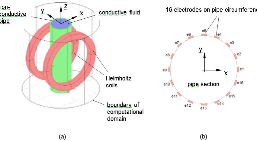
[image:5.595.81.507.73.307.2](a) (b)
Fig. 1: Electromagnetic flow meter; (a) geometry and computational domain; (b) position of
electrodes
The Fourier series expansion of the velocity field can be written in the form:
1
0 cos sin
2 1 ,
k
k k
z r c r c r k s r k
v (2.5)
where the coefficients are obtained as follows
1
, cos d 0,1,2,...2 0
v r k kr
ck z
(2.6)
1
, sin d 1,2,...2 0
v r k kr
sk z
(2.7)
The potential distribution (2.4) after substitution of the velocity field (2.5) will take the form:
1
1 1
0
1 cos cos 1 sin 1
k
k k k
k c k M s k
M c
M B
U (2.8)
with
d 0,1,2,...0
1
1
r k
R r r c c M
R k
k k
6
d 1,2,...0
1
1
r k
R r r s s M
R k
k k
k (2.10)
2.2 Conditions for a Given Polynomial Velocity Profile Component only Giving Rise to a Single
Discrete Fourier Transform (DFT) Component
The velocity profile is assumed in a polynomial form. For such functions the coefficients (2.6) and
(2.7), together with the potential distribution (2.8), can be determined analytically. The superposition
of polynomial components can also be used to approximate more complex velocity profiles. Since the
EMFM contains 16 electrodes (N = 16), as will be described in Section 4, polynomials up to 6th order
can be reconstructed after applying the Discrete Fourier Transform (see Section 2.3). Suppose the
nth-order component of the velocity profile (0n6) is in the simple form
Qn n Qn
nn n
R y x
a y x
[image:6.595.194.396.368.537.2]v ; cos
, sin
, (2.11)Fig. 2: Definition of the direction Q,n
with Q,n denoting the angle of direction with respect to the x-axis, where this component is defined,
and an is constant. The velocity component, vn, only changes in the direction Q,n and is constant
along lines orthogonal to this direction (see Fig. 2). It should be noted that Q,n is not defined for n =
0, because v0 = a0 for a uniform velocity profile. The potential distribution for this velocity component
7
2 0 , ,, cos 2 cos 2 1 sin 2 sin 2 1
1 2 1 1 n k n Q n Q n n n
n n k n k n k n k
k n BR a n
U (2.12)
where odd is for 2 1 even is for 2
2 n n
n n
n
(2.13)
The overall boundary potential distribution U~
is obtained by summing Un() for all individualvelocity components (e.g. 0n6). In this case, however, a given component of the DFT of U~
does not relate to a single velocity component, because each velocity component will give rise to
multiple frequencies in the boundary potential distribution (see Eq. (2.12)). In order to be able to
obtain information about the nth velocity component from the DFT, Un() must be expressed only in
terms of the trigonometric quantities, cos(n+1) and sin(n+1). This will ensure that in the case of several velocity components, each of different order n, the (n+1)th component in the DFT of U~
relates only to the nth order velocity component (see Section 2.3). For the nth order velocity
component, in order to eliminate terms other than cos(n+1) and sin(n+1), the velocity component has to be written in the form, if n is odd,
R y x a R y x a R y x a y xv Qn Qn
n n n n Q n Q n n n n n Q n Q n n n , , 1 , 2 2 , , 2 , , , , sin cos sin cos sin cos ;
(2.14)or, if n is even,
2
,02 , , 2 , , , , sin cos sin cos
; n n
n n Q n Q n n n n n Q n Q n n n a R y x a R y x a y x
v
(2.15)Thus, the nth velocity component is written as a sum of terms in the form of Eq. (2.14) or (2.15). The
coefficients an,n2, an,n4, …, an,1 or an,0 may be chosen so that the undesired trigonometric terms will
be eliminated. If m = n/2 (n is even) and m = (n–1)/2 (n is odd), then these conditions are as follows
n n n
n a
n
a, 2 ,
4 1 (2.16)
4 , 2 , 24 , 2 3 2 1 2 1 3
nn nn
8
... 2 3 2 3 2 1 1 1 2 1 2 1 1 2 1 2 1 4 , 4 2 2 , 2 2 , 2 2 , m m nn m nn m nn
n n a m n n m n a m n n m n a m n n m n a
2
, 2 11 1 2 1 2 1 2 1 2 1
ann m
m n m n m n (2.18)
In this case, the potential distribution associated with the nth velocity component will be simplified to
the following form which only contains terms in cos(n+1) and sin(n+1)
K
cosn , cos
n1
sinn , sin
n1
Un n Qn Qn (2.19)
where
a BRn
Kn n n,n
2 1 1
(2.20)
with B and R standing for the magnetic flux density and pipe radius, respectively. Note that in the
presence of multiple velocity components, the overall boundary potential distribution U~
is again given by summing the individual components Un() for all relevant values of n.The coefficient Kn can be obtained from the (n+1)th component Xn+1 of the DFT of the boundary
potential distribution U~
using 1 2 n n X K (2.21)Then, the coefficient an,n is determined from Xn+1 as follows
For uniform (n = 0) and linear (n = 1) terms, one possibility exists only:
1
10 , 0 2 Re sgn X BR X
a (2.22)
2 1 , 1 8 X BR
a (2.23)
For quadratic (n = 2) and higher-order (n > 2) terms:
1 1 , 2 1 n n
n
n X
BR n
a (2.24)
2.3 Application of the DFT to the Boundary Potential Distribution
9
potential Up (p = 0,…,N-1) at the positions of the measurement electrodes. The DFT of the series Up
then provides a series of N complex numbers as follows
2 /
0,1,..., 1 exp1 1 0
N n
N np j U
N X
N
p p
n
(2.25)where N is the number of samples. Note that Xn is associated with the (n-1)th boundary potential
component Un1
which is in turn associated with (n-1)th velocity component vn1
x;y . The value of Xn is related to the amplitude and phase of Un1
. Note also that Un1
has a wavelength of 2R/n. Thus, from the preceding arguments, a uniform velocity component v0
x;y gives rise to the boundarypotential component U0
which undergoes one complete cycle around the boundary. The DFT component associated with this uniform velocity component is X1. A linear velocity component
xyv1 ; gives rise to a boundary potential component U1
which undergoes two complete cycles around the boundary, etc. In case of a multi-electrode EMFM, N is equal to the number of electrodeson the circumference. The argument n associated with the complex number Xn is determined using
nn n
X X
Re Im arctan
(2.26)
taking into account the quadrant in which Xn lies. Unique values of Xn exist only up to the Nyquist
frequency, that is half of the sampling frequency (i.e. N/2). The numbers X0 and XN/2 are real; thus, the
numbers from X1 to XN/21 provide information about polynomial components of the velocity profile
from 0th (uniform) to (N/2-2)th order.
2.4 Angle of Direction of Velocity Profile
If the velocity profile takes the form (2.14) or (2.15), then the angle Q,n of the direction of velocity
component vn can be determined, as follows, from the argument n of the complex number Xn.
If n is odd and an > 0:
n k n
n n Q
1 2
,
n k n
k
n Q
, 2 1 , 2 1 k = 0,1,…,n–1 (2.27)
If n is odd and an < 0: the same solutions can be obtained, i.e. there are no further solutions.
10
nk n
n n Q
1 2
,
n k n
k
n Q
, 2 1 , 2 1 k = 0,1,…,n/2–1 (2.28)
If n is even and an < 0:
n k n
n n Q
1 2 1
,
n k n k
n Q
, 2 , 12 k = 0,1,…,n/2–1 (2.29)
The equations (2.27) or (2.28)-(2.29) imply that there exist n possible values of Q,n for a velocity
component in the form of an nth order polynomial. Consequently, if a velocity profile is composed of
the sum of velocity components up to the nth order polynomial, the number of possible solutions for
this velocity profile is n! Selection of the optimum solution is described in Section 3.2.
3. Procedure for Reconstruction of Velocity Profiles
3.1 Reconstruction of possible velocity profiles
The procedure to determine the polynomial components of a velocity profile and their directions is
summarized by the following stages.
The nth order polynomial component of the velocity profile is assumed in the form of (2.14) or
(2.15) if n is odd or even, respectively.
The measured overall potential distribution U~
can be written as the sum of a series of components Un
given by Eq. (2.19) with (2.20). For a 16-electrode EMFM the maximumallowable value of n is 6 (see Section 2.3), but, if required, n may be limited to a lower value nmax if
it is deemed unlikely that the velocity profile will contain velocity components of order greater than
nmax.
The DFT of the measured potential distribution U~
is obtained giving the DFT components Xn (n= 1,…,nmax+1).
The coefficient an,n is obtained from one of Eqs. (2.22)-(2.24).
The coefficients an,n2, …, an,n2m are calculated from Eqs. (2.16)-(2.18).
The possible angles of direction of the nth velocity component are determined from the argument
n+1 associated with the (n+1)th DFT component Xn+1 from Eq. (2.27) if n is odd, or from Eqs.
11
3.2 Choice of optimum solutionThe procedure as described in Section 3.1 provides n! velocity profile solutions if all velocity
components up to nth order are present. Thus, the optimum solution must be chosen from them. A
method is proposed in this study for this purpose, which is applicable for single and two-phase flows,
and is based on predicting the boundary potential distribution in a non-uniform magnetic field for a
given velocity profile using weight values. This non-uniform magnetic field is described later in the
present section and shown in Fig. 3b.
This method can be applied to choose the optimum solution if the potential distribution is
measured in a specific non-uniform magnetic field, as well as the uniform magnetic field, and the
potential distribution is calculated using weight values for all of the possible velocity profile solutions in
this non-uniform magnetic field. The optimum velocity profile is that for which the calculated boundary
potential distribution most closely matches the measured boundary potential distribution in the
non-uniform magnetic field. Before the potential distribution associated with a given velocity profile can be
calculated for the non-uniform magnetic field, the relevant weight values must be determined.
In the present study, the pipe section is divided into M subdomains (see Fig. 3a, from which it can
be seen that M = 30). For an N-electrode system the potential difference Uˆj between the jth electrode
and a reference electrode in the non-uniform magnetic field can be expressed as follows
1 ,..., 1 2
ˆ
1
N j
A w v R B U
M
i
i ij i op j
(3.1)
where Ai is the area of the ith subdomain and vi is the mean axial velocity in the ith subdomain
calculated using the analytical expression for velocity profile associated with one of the n! possible
velocity profile solutions. wij is the weight value relating the velocity in the ith subdomain to the jth
potential difference measurement Uˆ , j R is the internal pipe radius and Bop is a reference magnetic
flux density at a specific location in the flow cross section for the case of the non-uniform magnetic
field.
In this paper simulation results are presented whereby a reference velocity profile is entered into a
12
on the 16 electrodes are calculated in a uniform magnetic field of 0.01 T allowing the n! possible
predictions of the original reference velocity profile to be calculated as described in Section 3.1. (Note
that the uniform magnetic field is obtained by letting equal current of appropriate magnitude flow in the
same direction in each of the coils forming the Helmholtz coil).
Next, the same velocity profile is entered into COMSOL but for the case of a non-uniform magnetic
field, generated by letting currents of equal magnitude flow in opposite directions in each of the coils
forming the Helmholtz coil. The resultant non-uniform magnetic field is shown in Fig. 3b. The value of
Bop in Eq. (3.1) is arbitrarily taken as the magnetic flux density at electrode e13 (Fig. 1b) and in the
simulations described in this paper was equal to 0.005 T. For this non-uniform magnetic field the
potentials Up on each of the 16 electrodes were calculated using COMSOL, and 15 reference
potential differences Uˆj,ref (j = 1 to 15) were obtained by subtracting the value of the potential U5 (on
reference electrode e5) from the value of the potential on each of the remaining electrodes. Next, for
each of the n! velocity profile solutions, the 15 potential differences Uˆ were calculated for the non-j
uniform magnetic field using the weight value method encapsulated by Eq. (3.1). Finally, for each of
the n! velocity profile solutions, a quantity SU was calculated where
15
1
2
, ˆ
ˆ
j
j ref j
U U U
S (3.2)
The optimum velocity profile from the n! possible solutions was taken as that for which the quantity SU
was a minimum, i.e. the velocity profile for which the predicted potential differences using Eq. (3.1)
gave the best agreement with the calculated potential differences Uˆj,ref which were obtained by
applying the reference velocity profile to the COMSOL simulation model.
The weight values wij in Eq. (3.1) were obtained using a method described in detail by
Leeungculsatien & Lucas (2013). This method requires 30 separate COMSOL simulations, one for
each of the 30 subdomains shown in Fig. 3a. Each simulation was carried out using the non-uniform
magnetic field shown in Fig. 3b and for a given simulation the axial velocity in the chosen subdomain
(with index i) was set equal to vwt,i whilst the axial velocity in all of the other subdomains was set equal
to zero. The potentials on each of the 16 electrodes calculated using COMSOL were used to generate
13
from the potentials on each of the remaining electrodes. The weight values wij associated with the
chosen subdomain with index i were then calculated using the expression
15 ,..., 1 ; 30 ,..., 1 ˆ
2 ,
,
i j
v A
U B
R w
i wt i
j wt op ij
(3.3)
This process was repeated for the remaining subdomains, thereby allowing the 450 weight values
required for the correct application of Eq. (3.1), to be calculated. Due to the high computing time
required to calculate the weight values for each subdomain, the number of subdomains was limited to
30 in the present study.
In practical applications of the technique described above measured potentials, obtained from a
real EMFM in a uniform magnetic field, are used to generate the n! possible velocity profile solutions.
Similarly, measured potentials obtained from the EMFM in a non-uniform magnetic field are used for
selecting the optimum velocity profile solution using the weight value method described above. For a
given design of EMFM it is only necessary to calculate the weight values once, i.e. prior to the device
being used for the first time.
4. Electromagnetic Flow Meter
The geometry of the EMFM considered in the simulations described in this paper is given in this
section. It consists of a polytetrafluoroethylene flow pipe mounted within a Helmholtz coil (see Fig.
1a). The inner diameter of the pipe is 80 mm, and the thickness of the pipe wall is 5 mm. The inner
and outer diameters of the two coils forming the Helmholtz coil are 204.8 mm and 255 mm,
respectively. The potential distribution is measured by means of 16 electrodes that are placed at
angular intervals of 22.5 degrees on the pipe circumference as shown in Fig. 1b.
When the weight value method is applied for this specific EMFM, the specifications given in
Section 3.2 are considered. Since electrode e13 is located at the position x = 0, y = –40 mm (see Fig.
14
[image:14.595.91.501.70.283.2](a) (b)
Fig. 3: Specifications when applying the weight value method, (a) division of pipe section (h = (2*R)/6,
w = (2*R)/5, w1 = (2*r1)/5, where r1 = 29.8 mm for a 40-mm-radius pipe), (b) non-uniform magnetic
field, colour bar is in T
5. Application of Reconstruction Method
The method applied in this section is to reconstruct different velocity profiles. In this study,
COMSOL Multiphysics (COMSOL, 2008) is used to model the physical specifications of the EMFM
and to simulate the measurements. The computational domain is shown in Fig. 1a. It should be noted
that the pipe was not simulated in its full length in order to reduce computational cost. For each case
under consideration, a velocity profile is defined as the input for the COMSOL simulation. The
simulation then produces a potential distribution on the internal circumference of the pipe. This
potential distribution is used in the reconstruction method described in Section 3 to attempt to
reproduce the velocity profile that was initially input into the COMSOL simulation. The reconstruction
method was implemented in Matlab.
First, the reconstruction of possible solutions was tested by a known velocity profile defined in
polynomial form. Then, the method including the choice of optimum solution was applied to two more
complex velocity profiles which had previously been measured in two-phase flows.
5.1 Reconstruction of a quartic velocity profile
The following 4th-order (quartic) polynomial velocity profile was used for testing the reconstruction
15
x y v
x y v
xy v
x y v
xy v
xyv ; 0 ; 1 ; 2 ; 3 ; 4 ; (5.1)
where the indices refer to the order of polynomial, and the components are defined as follows
; 10 xy
v
90 sin 90 cos 1 ; 1 R y R x y x v
; 1 cos45 sin45 0.252
2
R y R x y x v
20 sin 20 cos 5 . 0 20 sin 20 cos 1 ; 3 3 R y R x R y R x y x v
; 1 cos0 sin0 0.75 cos0 sin0 0.06252 4
4
R y R x R y R x y x v
The reference velocity profile defined by Eq. (5.1) is introduced into COMSOL, and the potential
distribution in the uniform magnetic field is determined (Fig. 4a). This distribution is used as an input
for the reconstruction method to determine the possible solutions for the velocity profile. Since a
quartic velocity profile is the subject of reconstruction, the highest order of polynomial component is 4
and the number of possible solutions is 4! = 24. Then, the potential distribution in the non-uniform
magnetic field is determined by COMSOL for the original velocity profile. 24 possible solutions for the
boundary potential distribution in the non-uniform magnetic field are also calculated using the weight
value method given in Section 3.2. The sum of differences SU as defined by Eq. (3.2), is calculated for
each of the 24 possible velocity profile solutions, and the optimum velocity profile is the one for which
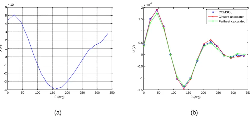
SU has a minimum value. Fig. 4b shows potential distributions obtained in the non-uniform magnetic
field: the distribution simulated by COMSOL is indicated by “COMSOL”, the optimum velocity profile
solution chosen as explained above is indicated by “Closest calculated”, and the solution for which SU
is maximum is indicated by “Farthest calculated”. It can clearly be seen that, although both calculated
potential distributions are close to that obtained from COMSOL, the “Closest calculated” shows a
closer agreement with the COMSOL one than the “Farthest calculated”; the quantity SU is 2.95108
and 8
10 87 .
8 for the “Closest calculated” and “Farthest calculated” velocity profiles respectively. The
corresponding three velocity profiles are drawn in Fig. 5. The chosen solution coincides closely with
the reference solution, although some minor differences are visible. However, the farthest calculated
16
0 50 100 150 200 250 300 350
-4 -3 -2 -1 0 1 2 3 4 5 6x 10
-4
(deg)
U
(
V
)
0 50 100 150 200 250 300 350
-1.5 -1 -0.5 0 0.5 1 1.5
2x 10 -4
(deg)
U
(
V
)
COMSOL Closest calculated Farthest calculated
[image:16.595.89.505.73.270.2](a) (b)
Fig. 4: Potential distribution of simulated and reconstructed quartic polynomial velocity profiles; (a)
uniform magnetic field; (b) non-uniform magnetic field
The reliability of the method may be evaluated by calculating a term v which represents an average percentage deviation in the local velocity of a reconstructed velocity profile as compared with
the original velocity profile. This term v is determined for each velocity profile solution according to Eq. (5.2):
100%~
min , max , ~
1 ,
min , max ,
in in
M
i
i in i
in in
average
v v
M
v v
v v
v v
(5.2)
Here, M~ is a number of subregions into which the cross section can be divided and where the velocity is calculated. In this case, M~ can be chosen arbitrarily high, because both the input and reconstructed velocity profiles are known analytically. In the example given here M~ was chosen to be 88. vin,i is the input velocity in the ith subregion. vin,max and vin,min are, respectively, the maximum and
minimum velocities in the input velocity profile. [Note that vin,maxvin,min is used in the denominator of
Eq. (5.2) rather than vin,i to prevent v tending to
for vin,i values which approach zero]. For the17
-0.04 -0.02 0 0.02 0.04 -0.04 -0.02 0 0.02 0.04 -1 0 1 2 3 x y -1 -0.5 0 0.5 1 1.5 2 2.5 3 -0.04 -0.02 0 0.02 0.04 -0.04 -0.02 0 0.02 0.04 -1 0 1 2 3 x y -1 -0.5 0 0.5 1 1.5 2 2.5 3 -0.04 -0.02 0 0.02 0.04 -0.04 -0.02 0 0.02 0.04 -1 0 1 2 3 x y -1 -0.5 0 0.5 1 1.5 2 2.5 3 [image:17.595.91.508.75.208.2](a) (b) (c)
Fig. 5: Simulated and reconstructed quartic polynomial velocity profiles, x and y are in m, colour bar is
in m/s; (a) reference velocity profile; (b) chosen optimum (closest calculated); (c) farthest calculated
The robustness of the method was studied by adding “noise” to the potential distributions obtained
in both the uniform and non-uniform magnetic fields. A random error of up to 0.01u was added to
the calculated true potential at each electrode, using COMSOL for the uniform magnetic field, where
u = 9104 V. The value of u was chosen because it represents the difference between the true
maximum and true minimum electrode potentials in the uniform magnetic field. [Note that this random,
absolute error represents a percentage error of up to about 2% of the true electrode potential for
those electrodes with the highest magnitude flow induced potentials. However, for those electrodes
with lower magnitude flow induced potentials, the percentage error of the true electrode potential,
caused by the addition of 0.01u, may exceed 10%]. Similarly a random error of up to 0.01nu
was added to the true potential at each electrode, calculated using COMSOL for the non-uniform
magnetic field, where nu =
4
10 3 .
3 V. The value of nu was chosen because it represents the
difference between the true maximum and true minimum electrode potentials in the non-uniform
magnetic field. Next, the reconstruction method was applied using these “noisy” potential distributions,
and the value of v was calculated using Eq. (5.2). This process was repeated over 20 trials, since the “noisy” potential distributions, and consequently v, are slightly different in each trial. The average value of v in these trials was 4.0%, with a minimum of 2.6%, and a maximum of 5.9%. Note that the
v value was 2.4% for the noise-free potential distributions. These results demonstrate that, for a future practical system, provided that the electrode potentials can be measured to an accuracy of
u
01 . 0
18
deviation v (Eq. (5.2)) in the local velocity will be of the order of only 4%. In what follows, the reliability of the method will be tested on velocity profiles that are not exactly polynomial.
5.2 Reconstruction of velocity profile measured in two-phase flows
The reconstruction method is applied in this section for two measured velocity profiles, namely the
water velocity profile in a two-phase flow of oil in water and the water velocity profile in a two-phase
flow of solids in water.
5.2.1 Two-phase flow of oil in water
Two-phase flow of oil in water in a pipe with inclination angle of 30 deg to the vertical was considered
in Zhao & Lucas (2011). They measured the volumetric flow rate of water Qw and of oil Qo, the time
averaged distribution of the local oil volume fraction o and the time averaged distribution of the local
axial oil velocity vo, as shown in Fig. 6. The local water velocity vw is calculated from the local oil
velocity vo using
slip o w v v
v (5.3)
where the axial slip velocity vslip in a pipe with inclination angle of 30 deg to the vertical is assumed to
be given by
30 cos
0 ,
slip slip v
v (5.4)
The value for vslip,0 was obtained experimentally as 0.16 m/s (Zhao & Lucas, 2011), hence vslip= 0.14
m/s. The input water velocity data in reduced spatial resolution as entered into COMSOL is shown in
Fig. 7a. The differences between Figs. 6b and 7a are that the constant slip velocity given by Eq. (5.4)
is subtracted and that the spatial resolution is reduced in Fig. 7a. The input velocity profile for the
COMSOL simulation shown in Fig. 7a is defined as follows. An 80-mm x 80-mm rectangular section
including the circular pipe is divided into 100 identical regions. Three regions at each corner of the
rectangular section fall outside the pipe where the velocity is zero (entirely white rectangles in Fig.
7a), and average water velocities were defined in the remaining 88 regions. Of each region, only the
area that falls inside the pipe is considered in the calculation (non-white areas of rectangles in Fig.
7a). Average velocities in each region are determined in correspondence with measured values.
19
that is used in the reconstruction is obtained from a COMSOL simulation in a uniform magnetic field
(see also Fig. 7b) using the input velocity profile described above as shown in Fig. 7a.
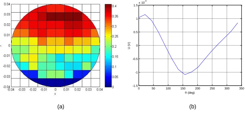
[image:19.595.95.518.141.333.2](a) (b)
Fig. 6: Measurements in a two-phase flow of oil-in-water in a pipe with inclination angle of 30 deg
to the vertical (from Zhao & Lucas, 2011), horizontal and vertical axes are in m, (a) time averaged
distribution of the local oil volume fraction, colour bar represents fraction, (b) time averaged
distribution of the local axial oil velocity, colour bar is in m/s
0 50 100 150 200 250 300 350
-1.5 -1 -0.5 0 0.5 1 1.5x 10
-4
(deg)
U
(
V
)
(a) (b)
Fig. 7. (a) Division of pipe section and the discrete input water velocity profile, x and y are in m, colour
[image:19.595.78.507.459.664.2]20
A preliminary study was undertaken to investigate the highest order polynomial velocity component
that should be used in the velocity profile reconstruction. To this end, the highest order component
was successively changed from first order, to second, to fourth to sixth order. For the velocity profile
containing velocity components up to first order only one solution exists, whereas in the other three
cases, multiple velocity profile solutions exist. For each case, the solution for which v, as defined by Eq. (5.2), was a minimum was chosen. These resultant velocity profiles are shown in Fig. 8. The
values of v for these four profiles are 11.01%, 9.02%, 6.75% and 7.91% (for highest order velocity components of first order, second order, fourth order and sixth order, respectively). Inspection of Fig.
8 shows that the velocity profile containing components up to sixth order displays physically
unrealistic spatial variations which were are also discrepant with the input velocity profile (Fig. 7a).
Note that an earlier series of simulations with a variety of input velocity profiles also showed that, for
velocity components of higher order than fourth, v values started to increase showing that the velocity profile was becoming less accurate. A probable explanation of this observation lies in the
tendency of the relative magnitude of DFT components to decrease with increasing ‘component
number’ - the magnitude of the 7th
DFT component (corresponding to the 6th order velocity component) being 2 to 3 orders of magnitude smaller than the first components (corresponding to the
lowest order velocity components). Thus, noise from any source (numerical or experimental), has a
significant effect on the calculated highest order velocity components. Until these noise sources are
better understood, the authors have decided to limit the highest order velocity component to fourth
order. Consequently, in the analyses which follow, velocity component terms up to fourth order only
will be considered.
-0.04 -0.02
0 0.02
0.04
-0.04 -0.02 0 0.02 0.04
0 0.1 0.2 0.3 0.4 0.5
x y
0.05 0.1 0.15 0.2 0.25 0.3 0.35 0.4 0.45
-0.04 -0.02
0 0.02
0.04
-0.04 -0.02 0 0.02 0.04
0 0.1 0.2 0.3 0.4 0.5
x y
21
(a) (b)
-0.04 -0.02
0 0.02
0.04
-0.04 -0.02 0 0.02 0.04
0 0.1 0.2 0.3 0.4 0.5
x y
0.05 0.1 0.15 0.2 0.25 0.3 0.35 0.4 0.45
-0.04 -0.02
0 0.02
0.04
-0.04 -0.02 0 0.02 0.04
0 0.1 0.2 0.3 0.4 0.5
x y
0.05 0.1 0.15 0.2 0.25 0.3 0.35 0.4 0.45
[image:21.595.87.506.69.289.2](c) (d)
Fig. 8: Reconstructed water velocity profiles with highest-order terms (a) 1st order, (b) 2nd order, (c) 4th
order, (d) 6th order, x and y are in m, colour bar is in m/s
Using the boundary potential distribution of Fig. 7b, the reconstruction method described in Section
3 was applied to determine the 24 possible water velocity profile solutions. The weight value method
described in Section 3.2 (and also in Section 5.1) was then used in order to select the optimum water
velocity profile. The optimum oil velocity profile can be obtained by adding the slip velocity vslip to the
optimum water velocity profile. It can be seen in Fig. 9 that the potential distribution for the chosen
water velocity profile solution (“Closest calculated”) provides a closer agreement with the reference
water velocity profile than the “Farthest calculated”. Note also that the quantity SU is
9
10 80 .
2 and 9
10 01 .
5 for the “Closest calculated” and “Farthest calculated” profiles respectively. However, the difference between the “closest” and “farthest” solutions is less than the difference between the
chosen (“Closest calculated”) and the reference solutions. The original and the chosen oil velocity
profiles are shown in Figs. 10a and 10b, respectively. The term v as defined by Eq. (5.2) is lowest for the oil velocity profile solution shown in Fig. 10c, whereas it is greatest for the solution shown in Fig.
10d. Consequently, a solution (Fig. 10c) closer to the original oil velocity profile than the chosen
22
closely the main characteristics in the original oil velocity profile, without being able to predict some of
the more subtle details that are visible in Fig. 10a.
0 50 100 150 200 250 300 350
-4 -3 -2 -1 0 1 2 3 4x 10
-5
(deg)
U
(
V
)
[image:22.595.201.391.146.307.2]COMSOL Closest calculated Farthest calculated
Fig. 9: Potential distribution of simulated and reconstructed velocity profiles in non-uniform magnetic
field
-0.04 -0.03 -0.02 -0.01 0 0.01 0.02 0.03 0.04 -0.04
-0.03 -0.02 -0.01 0 0.01 0.02 0.03 0.04
x
y
0.15 0.2 0.25 0.3 0.35 0.4 0.45 0.5 0.55
(a) (b)
-0.04 -0.03 -0.02 -0.01 0 0.01 0.02 0.03 0.04 -0.04
-0.03 -0.02 -0.01 0 0.01 0.02 0.03 0.04
x
y
0.15 0.2 0.25 0.3 0.35 0.4 0.45 0.5 0.55
-0.04 -0.03 -0.02 -0.01 0 0.01 0.02 0.03 0.04 -0.04
-0.03 -0.02 -0.01 0 0.01 0.02 0.03 0.04
x
y
0.15 0.2 0.25 0.3 0.35 0.4 0.45 0.5 0.55
23
Fig. 10: Oil velocity profiles, x and y are in m, colour bar is in m/s, (a) original from measurement; (b)
chosen by comparing potential distributions (min SU); (c) lowest value of v (Eq. 5.2), (d) highest value
of v
5.2.2 Two-phase flow of solids in water
The solids velocity profile for a two-phase flow of solids in water in an inclined pipe with inclination
angle of 30 deg to the vertical was measured in Cory (1999). The measured solids velocity profile is
shown in Fig. 11. The water velocity profile can be determined from the measured solids velocity
profile using Eq. (5.3) with oil velocity vo replaced by solids velocity. The slip velocity of the solids with
respect to water in a vertical pipe was found by Cory (1999) to be vslip,0 0.16m/s. This value is
negative since the solids density was greater than that of water. The application of Eq. (5.4) provides
the solids slip velocity in the inclined pipe as vslip 0.14m/s. The division of pipe section into a
number of regions in order to provide the input water velocity profile for a COMSOL simulation was
performed in the same way as explained in Section 5.2.1. Potential distributions were obtained from
this COMSOL simulation for both the uniform and non-uniform magnetic fields described in Section
[image:23.595.193.407.461.605.2]3.2.
Fig. 11: Measured solids velocity profile (from Cory, 1999)
For the reconstruction procedure water velocity profiles containing polynomial components up to
fourth order were considered. The optimum water velocity profile from the 24 possible solutions was
chosen by comparing the potential distributions calculated using the weight value method for the
uniform magnetic field with the reference potential distribution obtained from COMSOL in the
24
calculated”) provides a closer agreement with the COMSOL simulation than the “Farthest calculated”.
Note also that the quantity SU is
8
10 85 .
2 and 5.55108 for the “Closest calculated” and “Farthest
calculated” solutions respectively. The difference between the “closest” and “farthest” potential
distributions is less at some angular positions (270-350 deg) than the difference between the “chosen”
and the reference potential distributions. However, in this example there are some angular positions
where this situation is reversed (20-50 deg, 120-240 deg). The original, “closest calculated” and
“farthest calculated” water velocity profiles are shown in Figs. 13a, 13c and 13d, respectively. Also
shown, in Fig. 13b, is the water velocity profile for which v (Eq. 5.2) is a minimum. Similar conclusions can be drawn from Fig. 13 as from Fig. 10 in the previous example. The chosen (“closest
calculated”) solution (Fig. 13c) provides a visibly closer approximation to the reference water velocity
profile (Fig. 13a) than the “farthest calculated” (Fig. 13d). However, the value of v is lowest for the solution in Fig. 13b, i.e. a solution closer to the original water velocity profile than the “chosen” water
velocity profile exists. The value of v for the profile in Fig. 13b is 5.0%, whereas v = 5.2% for the chosen solution in Fig. 13c.
0 50 100 150 200 250 300 350
-1 -0.8 -0.6 -0.4 -0.2 0 0.2 0.4 0.6 0.8
1x 10 -4
(deg)
U
(
V
)
[image:24.595.197.391.407.568.2]COMSOL Closest calculated Farthest calculated
Fig. 12: Potential distribution of simulated and reconstructed water velocity profiles in non-uniform
25
(a)
(b)
[image:25.595.89.503.78.491.2](c)
(d)
Fig. 13: Water velocity profiles; (a) original as defined in COMSOL simulation; (b) lowest value of v (Eq. 5.2), (c) “closest calculated” solution by comparing potential distributions (min SU), (d) “farthest
calculated” solution by comparing potential distributions (max SU)
The results for the two examples presented in this section show that the method proposed for
choosing the optimum solution does not necessarily provide the solution with the closest velocity
profile to the original velocity profile. However, the chosen solution in both examples provides an
estimation of the reference velocity profile for which the mean deviation v (Eq. 5.2) is below 10%. For many industrial multiphase flow measurement applications this level of error would be acceptable.
26
An analytical velocity reconstruction method has been developed and tested, which is applicable to
flow measurement with a multi-electrode electromagnetic flow meter (EMFM). The method is based
on the Discrete Fourier Transform (DFT), and includes two steps. Firstly, possible solutions are
determined in polynomial form and secondly the optimum velocity profile is chosen from among them.
The first step requires measurement of potential distribution in a uniform magnetic field; whereas
measurement of potential distribution in a non-uniform magnetic field is necessary for the second
step. It was shown that the complex numbers obtained from the DFT coefficients provide information
about the coefficients of the polynomial velocity components of the reconstructed velocity profile,
together with the angle of the direction of these velocity components. Thus, a method has been
proposed that provides the velocity distribution analytically for a continuous conductive phase in a
circular pipe section, in either single phase or multiphase flow.
The application of the method to artificial velocity profiles constructed from polynomial velocity
components shows that the reconstructed velocity profile coincides closely with the original profile, in
spite of the fact that there exist multiple solutions with identical potential distributions in a uniform
magnetic field and with nearly identical potential distributions in the non-uniform magnetic field. When
the method is applied to more complex velocity profiles, then the choice among the possible solutions
may not be that which is closest by local velocities, i.e. that for which the term v is minimum. However, the chosen solution is a satisfactory estimation of the input velocity profile with a value of v that in general is not greater than 10%.
References
Bevir, M.K. (1970) The theory of induced voltage electromagnetic flowmeters, J. Fluid Mech., 43(3),
577-590.
COMSOL Multiphysics User’s Guide, Version 3.5. COMSOL AB, 2008.
Cory, J. (1999) The Measurement of Volume Fraction and Velocity Profiles in Vertical and Inclined
Multiphase Flows, Ph.D. thesis, University of Huddersfield, Huddersfield, UK.
Horner, B., Mesch, F., Trachtler, A. (1996) A multi-sensor induction flowmeter reducing errors due to
non-axisymmetric flow profiles. Meas. Sci. Technol., 7, 354-360.
Leeungculsatien, T., Lucas, G.P. (2013) Measurement of Velocity Profiles in Multiphase Flow using a
27
Morse, P.M., Feshbach, H. (1953) Methods of Theoretical Physics, Part II, McGraw-Hill, New York,
NY.
Sakuratani, M., Honda, S. (2010) Partially Filled Flow Tomography with Electro-Magnetic Induction,
SICE Annual Conference 2010, Taipei, Taiwan, 2758-2762.
Shercliff, J.A. (1962) The Theory of Electromagnetic Flow-Measurement, Cambridge University Press,
Cambridge, UK.
Teshima, T., Honda, S., Tomita, Y. (1994) Electromagnetic Flowmeter with Multiple Poles and
Electrodes, Proc. IMTC ’94, Hamamatsu, Japan, THPM 1-5.
Xu, L.J., Li, X.M., Dong, F., Wang, Y., Xu, L.A. (2001) Optimum estimation of the mean flow velocity
for the multi-electrode inductance flowmeter, Measurement Science and Technology, 12,
1139-1146.
Xu, L., Wang, Y., Dong, F. (2004) On-Line Monitoring of Nonaxisymmetric Flow Profile with a
Multielectrode Inductance Flowmeter, IEEE Transactions on Instrumentation and Measurement,
53(4), 1321-1326.
Zhang, Z., Lucas, G.P. (2013) Determination of power law velocity profiles by electromagnetic flow
measurement. Proc. 7th World Congress on Industrial Process Tomography (WCIPT7), Krakow,
Poland, 747-756.
Zhao, X., Lucas, G.P. (2011) Use of a novel dual-sensor probe array and electrical resistance
tomography for characterisation of the mean and time-dependent properties of inclined, bubbly