A structured approach to web panel surveys: the use of a sequential framework for non random survey sampling inference

(1)

The London School of Economics and Political Science

A Structured Approach to Web Panel Surveys

The Use of a Sequential Framework for non-Random Survey

Sampling Inference

Yehuda Dayan

A thesis submitted to the Department of Statistics of the London

School of Economics for the degree of Doctor of Philosophy,

(2)

(3)

Declaration

I certify that the thesis I have presented for examination for the MPhil/PhD degree of the London School of Economics and Political Science is solely my own work other than where I have clearly indicated that it is the work of others (in which case the extent of any work carried out jointly by me and any other person is clearly identified in it).

The copyright of this thesis rests with the author. Quotation from it is permitted, provided that full acknowledgement is made. This thesis may not be reproduced without my prior written consent.

I warrant that this authorisation does not, to the best of my belief, infringe the rights of any third party.

(4)

Abstract

Web access panels are self selected panels constructed with the aim of drawing in-ference for general populations, including large segments of the population who rarely or never access the Internet. A common approach for modeling survey data collected over access panels is combing it with data collected by a randomly selected reference survey sample from the target population of Interest. The act of joining the panel is then treated as a random process where each member of the population has a positive probability of participating in the survey. The combined reference and panel survey sample can then be used for different esti-mation approaches which model either the selection process or the measurement of interest, or some case the two together. Most practitioners and academics who have considered this combined sample approach, model the selection process by a single phase process from the target population directly to the observed sample set.

In the following work, I assume selection into the panel is a sequential rather than a single phase process and offer several estimators that are underlined by appropriate sequential models. After a careful investigation of a variety of single phase methods applied in practice, I demonstrate the benefits a sequential frame-work has to the panel problem. One notable strength of this approach is that by assuming a sequential framework the modeler can include important variables associated with Internet and Web usage. Under a single phase model inclusion of such information would invalidate basic assumptions such as independence between selection and model covariates.

(5)

Acknowledgements

I would like to thank my supervisor, Professor Jouni Kuha, for his consistent support from the early stages of this research to the last days of writing this document. His sharp advice and confidence in my ability to complete this jour-ney has been invaluable. I also would like to thank wholeheartedly the LSE Department of Statistics who overlooked my part-time student status and have supported me with real generosity.

This research could not have happened without Karsten Shaw, Dr. David Herron and Dr. Patten Smith of Ipsos-MORI who provided financial and professional backing, as well as a significant level of flexibility at work to allow me to pursue this project.

Above all, I want to thank my parents, Yossi, Ayelet and Meyrav for their un-conditional love and support.

(6)

Chapter 1

Web Access Panels

1.1

Introduction and Opening Words

The expansion of Online research and Online survey research is a major trend in the past fifteen years. From a very small base Inside research (2009) put the US total Online research in 2009 at about $2 billion, while the UK market research society estimates that 26% of all research in the UK in 2010 was done Online. The Lion’s share of this research is done over the platform of Web panels. This is largely a replacement technology with 85% of the research conducted over these panels have been migrated from traditional research modes such as face to face or telephone. The main engine for this growth has been market research studies such as brand evaluation, product concept trails, advertising testing, customer satisfaction surveys. Political polling, always having an outsized influence1 _on

the research market and the public perception of research, has also shifted in-creasingly to Online platforms and has had a major part in a wider public and commercial acceptance of estimates based on Web panel data.

Panels can be recruited by means of traditional probability designs (such as the Knowledge Networks panel), however, the vast majority of panels are assembled through a non-probability and loosely controlled process. As means of recruit-ment panels employ a large range of procedures to solicit population members to join the panel. These offers normally suggest the prospect of receiving monetary remuneration for their survey response, but also stress social aspects such as the participation in public debate or the possibility of influencing the development of new products or improving relationships with companies. After joining, the panel collects profiling information such as social and demographic indicators as well as some attitudinal and behaviour information. The panel company then communicates with their members by email or when panelists actively log on to the panel website.

(10)

The non controlled and non-probability method of panel recruitment are in stark contrast to the conventional framework of survey sampling theory underlying much of the survey based research for over 50 years (Baker et al., 2010), and so it is not surprising the resistance Web panel faces from much of the key stake holders of the industry including the academic, governmental as well as the com-mercial communities. But given the deep societal changes of the last decade reflected in dramatic new methods of communication and social interactions, changes in consumer habits, as well as commercial pressures the march of sur-veys moving Online is inevitable.

However, this relatively fast shift in the adaptation of Web panels in the industry has exceeded the pace of methodological advancement. And while still fiercely debated in academia, Web panels are now an integral part of survey based re-search. Thus, it is necessary to acknowledge the importance of Web surveys, instead of neglecting their potentials by regarding them as a cheap and dirty method. It becomes now the methodologists responsibility to devise ways to improve and devise frameworks that can underline a statistical approach to Web panel based survey inference.

Luckily, there have been a number of substantial attempts by social scientists in the design aspect of Web surveys particularly in questionnaire design and us-ability issues. However, findings in these studies do not cover the full picture of Web survey methodology, as they are limited to improving the quality of data collected from persons who already participate in the surveys. At the same time, academic researchers have in recent years started investigating and publishing work on the topic and along with valuable work done in the commercial sector there exists a good initial body of empirical and theoretical work to build on.

Still, a great deal more is left to develop in the field and my hope is that this work may contribute to a more structured and detailed framework for the statistical inference of general population parameters based on Web panel survey sampling data.

1.2

Online Panels

(11)

platform is built on - the Internet2_{. When the target population of interest is}

certain classes of the population such as the student population or a commercial organization, this issue is of minor concern given their high Internet penetra-tion levels. However for general (e.g. napenetra-tional or internapenetra-tional) populapenetra-tions a non negligible and distinct segment of the population is not Online. Despite the digital revolution of the past decade and the seemingly omnipresence of the Internet in our daily lives in 2012 still only 76% of the EU population had used the internet at least once, while only 67.5% of the EU population are regular users - that is use the Internet at least one time a week (European Commission, 2013). In the US the Pew research center estimates that only 72% of Internet users go Online at least once a week (Rainie, 2010). Furthermore, the use of Internet is strongly associated with education level, income, profession, health disability and age: for example in the UK, while almost all people aged 16-44 have used the Internet, only 3 out of 10 people aged 75+ have (ONS 2014). In the US, demographic groups such as Hispanics and blacks are underrepresented in the Online population (Baker et al., 2010).

It is true that effectively all Internet users have an email account, but still there is no complete list of these addresses. Furthermore, while several Internet users may share a single email address, more and more commonly users acquire multi-ple email accounts from different providers which are used for different activities. Many of these addresses are forgotten, left unused without being disabled. In general , the non standardised format of emails blocks the possibility of establish-ing an Online equivalent of the telephone samplestablish-ing random digit dialestablish-ing (RDD) methodology. It is worth noting that even if a useful list of email account could be compiled, legal and commercial body regulations would block the use of such a list for privacy and consumer rights reasons (Baker et al., 2010).

The Online panel platform is a widely used solution to this lack of sampling frame or sampling methodology for general population research. The ISO 26362: Access Panels in Market, Opinion, and Social Research offers the following defini-tion of Online panels: “A sample database of potential respondents who declare that they will cooperate with future [online] data collection if selected” (Interna-tional Organization for Standardization 2009). This is a broad definition which can include (as noted in section 1.1) panel databases collected by an Offline ran-dom probability design as well as one that is collected through a non probability selection procedure - namely through a wide placement of Online ads and offers to join the panel and partake in future surveys.

A further distinction can be made by the population targeted for the panel based research. General Population panels are collected to correspond to the general population Online, or when census balanced, to represent the general

(12)

tion. Consumer Panels are similar but may be limited to certain ages (25-55) and demographics more relevant to market research exercises such as a study of the consumer packaged goods market. Sub-panels aim to represent certain sub-populations for which unambiguous features or attributes are available link-ing them to groups of panelist for specific areas of studies. One example is a Handicap or disability panel, where members of the general population panel can be identified as having a disability and can be gauged on unique health is-sues, social views, economic status and even shopping patterns. This is a cost effective way of researching such low incidence population segments. Similarly Specialty Panels and Business to Business (B2B) panels which aim to survey specific members of the population such as business executives legal profession-als, musicians, hunters and other members of the panel representing small, low incidence, groups of the population. Proprietary Panels are panels usually built and maintained by a research company but exclusively used by a certain com-pany for their own research needs. Banks, Content providers or large retailers with large customer databases are companies which benefit from owning a panel representing their client population.

As noted my research focuses on the problem of inference of general population statistics based on data collected from panels assembled Online through a non probability process, however, the ideas are immediately transferable to any of the above panel types.

1.3

Data-Collection Methods in the Face of

So-cial, Economic and Technological changes

The field of survey methodology and specifically its data collection and data measurement tools evolve dynamically along with the cultural and technological changes. The survey methodology field advances by expanding the variety of measurements of day to day activities and the views of the society it studies. Over the previous century, among the evolutions most notable in the field was the introduction of telephone interview (Groves and Kahn, 1979; Dillman, 1998; and Dillman, 2002). It is noteworthy then that when the idea of conducting sur-veys over telephone was first introduced, researchers were skeptical and not fully convinced of the effectiveness of the method. One possible explanation was the famous failed Literary Digest poll which was based as well on a list of telephone owners. It is also true that the prevailing belief at the time was that surveys should involve face-to-face interactions.

(13)

telephone survey methodology (e.g., Groves and Kahn, 1979). Meanwhile, an innovative concept of balancing survey costs and errors to the maximum degree has influenced researchers to design surveys within some fixed amount of budget - The total survey error paradigm (e.g., Groves, 1989). A well-defined probability sampling procedure by random digit dialing was developed for telephone surveys (e.g., Mitofsky, 1970; Waksberg, 1978; Lepkowski, 1988; Casady and Lepkowski, 1993). Inevitably, practical considerations and societal changes boosted the le-gitimacy of telephone interviews. For example, increased telephone usage and a lowered household contactability for face-to-face interviews due to an increase in female workforce and a decrease in household size have made surveys by tele-phone more feasible and cost-effective. Now, teletele-phone surveys are a standard data collection method in developed countries.

It is clear now that the digital revolution and the internet have created another significant societal change and with it another leap in the sources of measure-ment available. The internet is profoundly changing the way we communicate with one another and so, the survey research field is experiencing another chal-lenging transition into implementing Internet based surveys.

As noted already Web surveys3 have been both hyped for their capabilities and criticized for their limitations. However, to put this in historical perspective, it is instructive to return to what was written about telephone and mail surveys when they were still regarded as unproven survey methodologies. In 1978, Don Dillman, a noted authority on surveying, said the following about mail and tele-phone survey questionnaires: ’Neither mail nor teletele-phone has been considered anything more than a poor substitute...’ for the highly regarded face-to-face in-terview. At the time this view was probably justified, because the two methods had many deficiencies and problems. Surveys by mail typically elicited extremely low response rates, even with short questionnaires. Further, it was not possible to reach many people by mail questionnaires, and among those to whom ques-tionnaires could be delivered, the best educated were far more likely to respond. Even completed questionnaires left much to be desired in terms on non answered questions. It is not surprising, then, that users of the mail questionnaire treated response rates well below 50 percent as acceptable and explained away problems of data quality with disclaimers such as, this is the best we can expect from a mail questionnaire (Dillman, 1978, pp. 12).

Not unlike the situation with mail surveys in the 1970s, many questions and concerns exist about how to best conduct Web surveys and whether they are, in fact, scientifically valid. However, reflecting on Dillman quotation and making the necessary substitutions between web, mail and Web, the statement will

ac-3_{In Web surveys the respondent visits the survey Web site by either clicking a hyperlink in}

(14)

curately reflect much of the criticism directed at Internet-based surveys today. Therefore, it is inevitable to consider Internet surveys as an alternative or rather a new survey tool alongside traditional mail and phone survey methods.

More positively, Web-surveys do have advantages over more-traditional methods in certain applications, and the use of this medium will continue to expand. Com-pared to traditional survey platforms proponents argue (Kellner, 2008; Rivers, 2010) that: (1) they are less time consuming; (2) they are just as good or better than more-traditional surveys; (3) they are much cheaper to conduct; and (4) they are easier to execute. However, these assumptions may or may not be true depending on the individual circumstances of the survey. Therefore, researchers need to understand the current limitations of Web surveys.

According to Dillman (2002) our survey methods are more a dependent variable of society rather than an independent variable constructed by the survey com-munity in isolation. In fact the ideal survey methodology is likely to reflect the society and its culture. As Taylor and Terhanian (2003) argue, just as telephone surveys began to be adopted extensively a few decades ago mirroring the societal and technological trends, the survey methodology field is currently witnessing a widespread growth in the use of Web surveys. These changes are simply mani-festation of societal trends.

1.4

The Web access Panel- Mechanics and a

To-tal Error Perspective

Web access panels have their roots in the prior post-mail panels started by US market research companies, including Synovate, NOP and others (Baker et al., 2010). These mail panels were assembled by a non random processes, similar to the Web panels, but through non Internet sources. These panels were marketed by commercial research companies based on their superior speed, cost and ability to capture low incidence population - again similar to the strengths of today’s Web panels.

(15)

Population Coverage

Our interest is in estimating certain statistics of a target population. In sur-vey sampling theory a target population is a finite population of units, that is a population which at least in theory can be counted over a certain period of time and are thus observable. A classic example is a survey targeting the US population of adult household members in a certain month. Usually a target population is defined already while considering a sampling frame from which to collect population members. That is a researcher may want to survey the entire adult population, however technically and financially limiting the aim to the household member population is a more feasible proposition. Any sampling frame (e.g. the Postcode Address File in Great Britain) will have limitations that may cause errors in the eventual estimation stage. In traditional sampling frames these include undercoverage, such as non registered households but also overcoverage- caused by multiple mapping and duplications which usually are a function of several household members clustered under the same address. To deal with these issues the survey community established recognized and tested procedures to identify and minimize such problems

(16)

Recruitment, Registration and Profiling of Panelists

Non response or non cooperation is an error affecting any survey mode as it severs the link between the planned selection design from the actual sampling distribution. From the nature of Web access panels’ assembly procedure, which relies on a multitude of contact points with the target population (many of them loosely controlled by the panel management team), the magnitude and charac-teristics of such non cooperation with the collection process is significant.

The recruitment to the panel is mainly done Online, but can have an Offline ele-ment as well. Panel companies attempt to advertise and solicit volunteering to as many members of the population as possible. The extent of the recruitment drive is a function of the cost constraints and the desired social and demographic pro-file of the panelists. Motivation to join and participate in surveys can be driven by aspects such as monetary incentive - either fixed or contingent, the desire of the member for self-expression of certain views and influence public opinion, the opportunity to view survey results and as a means of entertainment. It may be somewhat surprising that when studying panelists’ motivation Poynter and Comley (2003) found a fairly even mix of the above list with monetary reward (42%) the highest stated, followed by curiosity (40%), entertainment (20%) and a desire for self expression of views (28%).

(17)

Given the uncontrolled nature of the process, it is almost impossible to estimate or even define the response rate of the overall selection process. In one such attempt Alvarez et. al, (2003) studied the case of Web banner recruitment and found that the recruitment rate per Web banner impression was 0.002% while the recruitment rate per actual Web banner ad click-through was just above 6%. Another study by the same authors found that a vendor email list com-piled through a co registration agreement yielded a 32% recruitment rate. This is one indication of the reason for the prevalence of vendor list based recruitment.

Baker et al. (2010) summarize several empirical evidence of the recruitment or self selection error for US and EU panels. The evaluations are conclusive in that population member who join Web access panels differ significantly from the general Online population. For example a study of a Dutch panel (Vonk et al. 2006) found it underrepresented ethnic minorities and immigrants while over represented frequent Internet users, voters for certain political parties and religious groups. Similar evidence has been documented by US studies (Krosnick and Chang, 2004; Chang and Krosnick, 2009; Dever et al., 2008; Couper, 2000, and others).

The majority of large commercial panels follow adouble opt-in procedure of join-ing the panel, which means that after the collection of a population member’s (email) address, the panel sends him or her an email offering to join the panel by following an attached link leading to the panel web site. On arrival most panel companies screen potential panelists through a recruitment questionnaire, recording a long list of profiling data which can range from basic social demo-graphic characteristics to attitudinal, behaviour and psychogrpahic4 information which in turn will be used to identify the overall profile of the panel as well as sampling covariates for specific survey studies. The profiling phase is used as well to maintain the integrity of the panel by means of different validation pro-cedures. The aim of these procedures is to prevent fraudsters from joining the panel and can include comparing profiling data to third party databases, checks on the stated home address against postal records and ISP address as well as data integrity evaluation (to test if the profession, age and other pieces of in-formation given are ’reasonable’) and digital fingerprinting to check for multiple registration (duplication tests) to the panel.

Incentive and Panel Maintenance

As is evident from the discussion above, acquiring a panelist is an expensive undertaking and so an important part of the management’s team resources is to decrease the level of panel attrition. This is a natural process which occurs in any panel, with the largest group of panel drop-outs in fact are the group of new

(18)

members. Longer term, attrition can be influenced by the length of the surveys taken, the topic of studies when they do not match the respondents interests, or inversely by a panel not being engaged enough in the sense that the member is not sent survey requests over a long period of time.

The vast majority of panels offer panelists incentives. A common incentive is to use redeemable points that are collected for each survey completed. The amount of points gained can be a function of survey characteristics such as the length of the survey or the perceived interest (or how tedious, boring) members may find answering the questions. Another factor is the panelist characteristics, where low incidence panel members (such as top business executives, members with a specific disability) will likely be offered a higher number of points for completion of the survey. Points can be redeemed in numerous ways: gift certificates or other forms of vouchers, cash by check or bank transfer, purchase services or products through participating websites, multiple participation in sweepstakes.

An important guiding principle the panel management must always follow is that regardless of the incentive method, the level of remuneration should be high enough to incentive panelists to participate, but must not be large enough to encourage population members for which panel membership is a major source of income, that is professional panelists, to be encouraged to join.

Within Panel Survey Sampling

Given the unrepresentativeness of the panels, it is uncommon for a researchers to design a simple random sample from the panel. More likely, panel manage-ment will sample by non random purposive methods. In the panel managemanage-ment terminology ’sampling is the process of drawing a sample from the panel that fulfills certain criteria, often referred to as quotas’ (Michael 2010). These criteria can be basic social demographic quotas taken from national statistic organiza-tions, but depending on the survey topic can include constraints on the sample based on lifestyle and attitudes, brand and category usage, ownership health conditions. To estimate the quotas necessary, several panel companies run in parallel a smaller ad hoc random reference survey to estimate the population distribution of these specific variables. Such reference surveys, for cost reasons, can also be conducted on an ongoing basis and used to design several surveys simultaneously. This approach was pioneered by Harris Interactive. Clearly, the reference survey must match in wording the panel survey questions and should be as much as possible mode and time insensitive.

(19)

traditional survey sampling world5 _{a strength of Online panels is their complete}

knowledge of the distribution of the panel members across the many profiling variables and the control on the distribution of the achieved sample. An inter-esting example of the use of this knowledge are political polls, where many panel companies at the time of a general (or in some cases local) elections, take a ’snap shot’ of the electorate map by surveying all panel members over the days before and after the election. Companies use this profiling data to anchor the panel to the correct political landscape which they can then use on an ongoing basis for political, social and even economic research.

1.5

Structure of Thesis

In chapter 1 I have introduced the idea of Web panels as a substitute to the classical survey sampling population frame. I also have described there the main methodological challenges practitioners face when using this new survey plat-form. In chapter 2 I review common approaches to the problem, beginning with the important fixed population framework. In chapter 2 I also explain the sta-tistical logic of common panel practices such as purposive and quota sampling. In chapter 3 I propose a sequential framework to the Web panel process and adapt the most common estimators reviewed in chapter 2 to the sequential case. I then discuss the strengths these estimators have compared to their single phase framework counterparts, and demonstrate these properties through several sim-ulation studies. In chapter 4 I introduce the idea of using a random reference random survey as a surrogate to the unknown general population distribution and describe how the sequential estimators of chapter 3 can be computed over a combined sample set collected over both Web panel and reference surveys. In the final sections of chapter 4 I move away from post survey adjustment methods and propose a within-panel sampling design, which aims to balance the achieved sample to a set of population statistics. I show that combining this balanced sampling design with estimators built over a combination of selection and measurement of interest models achieve an additional level of robustness to misspecification.

5_{Although there is a significant divergence across the Atlantic where in Europe quota}

(20)

Chapter 2

Modelling Panel Data

-Introduction to the Problem and

a Review of Relevant Approaches

2.1

Overview of Chapter

In chapter 1, I described the complex and to an extent intractable survey process of Web access panels. The objective of this expensive undertaking is to draw in-ference about the population from which the panelists originate. This fits the survey sampling problem of estimating population quantities from a subset of the population dataset, However, the non random and highly complex nature of the underlying selection and survey process, and the lack of (even a proxy) sampling frame stands out from the main stream of survey research datasets. It may be only a small exaggeration to state that since the inception of scientific survey sampling in the 1920s Web panel surveys are the first survey platform possessing such characteristics that have gained traction and have not been dis-missed outright by the research community.

(21)

strengths in the context of the Web panel survey sampling setting which I will try and highlight.

Even before, I can state that one common weakness of these approaches is that they usually reduce the complex survey selection process into a single model. More clearly, any inference over data collected from a sample of a population must address explicitly or implicitly the selection (or missingness) mechanism. It will be evident from the discussion that as a general rule, commonly used approaches model the panel selection mechanism as a one phase process, which from the short introduction it is clearly not to be the case. This reduction of what is a sequence of conditional processes into a one phase process, I will ar-gue, weakens both the ability of the analyst to offer a satisfactory model for the selection mechanism and may increase the likelihood of model misspecification of the measurement of interest - because it reduces artificially the complexity of the selection process, and prevents the use of valuable information which could otherwise be used directly.

A modelling framework which takes into account the sequential nature of the selection process will be given in the following chapter 3, while here I consider approaches which could be used if selection could be treated as being generated by a single phase mechanism.

In the following I start by setting up the notation and formalizing the basic problem, then section 2.3 discusses the applicability of the fixed population ap-proach of survey sampling inference to the Web panel problem. This is a natural starting point given the popularity of the framework in the survey community. Section 2.5 covers the ’translation’ of observational study methods, which are highly relevant to the Web problem, into the context and terminology of survey methodology. After this, over sections 2.7-2.9 I review separately common π,m

and πm-estimation procedures, their strengths and weaknesses - all within the context of the Web panel problem.

2.2

Notation, Terminology and Basic Set Up of

the Problem

A finite population s0 ₌_{₁_{, ..., k, ..., N}_} _{consists of}_{N <}_∞ _{units where}_k

repre-sents the kth _{unit of the population, a physically existing element on which we}

can make measurements or observations. For convenience, when describing basic results I assume that the size N, at least conceptually, is known.

(22)

asso-ciated with the kth _{unit of the population.} _When _y

k is in bold font then

yk = (y1k, ..., yQk)0, that is for each unit k sampled, a Q−vector of variables is

recorded - usually Qis of high dimension. The unknown set of population values is denoted in general by theN×Qmatrixys0 = [y₁, ...y_k, ...,y_N]

0

and in the case where only one variable is recorded by the N−vector ys0 = (y₁, ..., y_k, ..., y_N)

0

. When unambiguous, I may drop the s0 _{which here indicates the relevant set of}

population units. These study variables can be continuous, as in situations where

yqk,q = 1, .., Q stands for the ’income’ or ’hours listening to the radio’ of unit k

of the population. In many other cases, however, yqk is categorical , for

exam-ple a dichotomous variable such that yqk = 1 if k has the attribute ’The Times

reader’ and yqk = 0 ’Not The Times reader’. But for specific cases, we consider

our objective is in estimating linear functions of y such as the population mean y_s0 =N−1

P

s0yk.

In the most general setting we assume the value yk is a single draw from the

distribution of the possible outcomes and is therefore itself stochastic. The un-observed measurementsy= [y1, ...,yN]

0

, the fixed finite population, are assumed to be the realized outcome of random variablesY = [Y1, ...,YN]

0

, the Superpop-ulation, with joint distribution about which certain features are assumed known. This idea of a Superpopulation from which the finite population is a sample was first proposed by Deming and Stephan (1941).

Formally, let f(y) be the probability density function (for continuous random variables) or the probability function (for discrete random variables) of the Su-perpopulation distribution of the random variablesY. Normally when the values x = [x1, ...,xN]

0

of X an N ×P matrix with typical xk a P ×1 vector are (or

assumed) known for all members of the populations0 _{then I shall use the}

condi-tional density function f(y|x). In some cases I assume that the family of Super-population distributions is indexed by an unknown parameter θ = (θ1, ..., θT) of

finite dimensionT so that the densityf(y) is denotedf(y;θ) and the conditional density function is denoted f(y|x;θ).

The survey statistician observes only a subset of the population of interest. As noted above, selection is underlined by a sequence of panel processes, however, most published work on Online access panel data (for example see Isaksson et al., 2004; Lee, 2006; Rivers and Bailey, 2009 and Lee and Valliant, 2009) reduces this into a single selection model from finite population to the sample surveyed. This is the approach we take throughout this chapter, but will be relaxed in subse-quent chapters.

Formally let S = (S1, ..., SN)

0

be the N ×1 vector of indicator variables where

Sk = 1 if unit k belongs to the observed set and Sk = 0 otherwise, with

distri-bution P r(S =s) =p(s) where s = (s1, ..., sk, ..., sN)

0

(23)

population units participating in the survey, that is s = {k : Sk = 1}, then for

any selection mechanism with no duplication (such as discussed in this work), the event S =sis equivalent to the event S=sthat is P r(S =s) =P r(S=s). When necessary I associate with the selection distribution an unknown param-eter vector φ so we write p(s;φ) or p(s;φ) and when appropriate a conditional distribution p(s|x;φ) .

Givens, the populationyis partitioned ys0 = (y_s,y_s) wheres is the compliment

set of unselected population members. Throughout assume that the observed sample size P

k∈s0Sk = nS is large enough so that estimation and inference is

reasonable.

Throughout I assume exchangeability of p(s) and f(y) in the sense that all per-mutations, for example for (Sk1, ..., SkN), have the same N−dimensional

proba-bility distribution. In other words, the labels k are uninformative in the distri-bution. See Cassel et al. (1977, p.72) for a more detailed definition.

2.3

The Coverage Constraint of the Fixed

Pop-ulation Framework

As a survey sampling platform, an investigation of the Web access panel infer-ence problem should start with the fixed population approach which is practised by the overwhelming majority of survey statisticians. In the following I discuss briefly the inferential framework and evaluate the difficulty of implementing rele-vant estimation strategies in the panel context. I assume throughout this section a basic familiarity of the reader with the fixed population framework of survey sampling inference. Standard references for this idea is given by Cochran (1977), Cassel et al. (1992), S¨arndal et al. (1992) and Kish (1995).

In the fixed population approach all values of variables are considered fixed - but unknown - at the outset. Variables y and x are not random, and are variables only in the sense of taking possibly different values (S¨arndal et al., 1992, section 9.2). Fundamentally, randomness is due only to the subset selection process. The problem is that whatever modelling approach one takes within this framework, when tackling the panel question the researcher is constraint by the fact a subset of the population cannot be selected into the sampling set, resulting in a biased estimator.

Classically, it is understood that under a certain probability model p(·) we can state before selection the probability of observing unitss ⊆s0_{, the sample. More}

(24)

satisfiesp(s)≥0 ∀s∈ S and thatP

s∈Sp(s) = 1. An important element in fixed population statistical inference is the calculation of the inclusion probability of a random unit into the set s. For a given p(·),

πk = P r(k ∈S) that is P r(Sk = 1) =

X

S3k

p(S)

where the notation P

S3k is understood as the sum over all samples s which

include unit k of the population s0.

In fixed population inference, a selection model (or sampling design) is said to be measurable if πk > 0 and πkl = P r(k&l ∈ S) > 0 for all k, l ∈ s0. The

positive probability of selection for each unit is a necessary and sufficient condi-tion for the existence of unbiased estimators, while the positive joint probability for each pair of population units allows calculation of valid variance estimators, and using observed survey data, confidence intervals that achieve the theoretical coverage rate (see Lemma 3.4 in Cassel et al., 1977). Estimators are evaluated by properties such as expectation, variance, mean square error (MSE) which are all defined with reference to the specific selection model p(·).

Traditionally, the estimator accompanying the fixed population approach is the

HT-estimator (Horvitz and Thompson, 1952)

ˆ

y_s0 =N−1

X

k∈s0

Sk

yk

πk

=N−1X

k∈S

yk

πk

. (2.1)

A popular alternative replaces N by ˆN =P

sπ

−1

k .

Classical theory assumes that πk are known and specified by the researcher. In

Web panels, however, respondents self select into the panel. There is a rich academic and commercial literature dealing with self selection and unit non re-sponse in the survey sampling process. A popular approach is to describe the self selection as a separate conditional phase to the sampling design. That is, we assume first that a sample s1 is selected by known designp1(·), and subsets2

selects to respond to the survey questions with unknown response process p2(·)

with (conditional) unit selection probabilityπ2k =

P

k3s2p2(s2|s1) wheres2 ⊃s1.

After invoking two selection models estimator (2.1) is impractical1_{, and an}

ap-propriate estimator in this case is

ˆ

y_s0 =N−1

X

k∈S2

yk(π1kπ2k)−1. (2.2)

1_{Even if both phases mechanism are known as}_π

k is not easily defined- we need to know

p1(s1) for all s1 which in normal setting is available, but also for eachs1 we must know π2k

(25)

The two estimators (2.1) and (2.1) are mostly of not the same form as

πk = P r(k ∈s1)P r(k ∈s2|k ∈s1)

= π1k(πk/π1k)6=π1kπ2k

where the difference lies in conditioning the probability in selecting k to s2 _on

the observed set s1 _{rather than on the event that} _k _{is in the realized set} _s1_{. See}

S¨arndal et al. (1992, section 9.2) for further discussion.

A popular approach of estimating the self selection probabilities π2 is assuming

a response homogeneity groups (RHG) which states that s1 ₌ _∪Hs1 h=1s

1

h so that

π2k = π2h for any k ∈ sh1; h = 1, ..., Hs1. Let n₁ = ∪ H_s1

h=1n1h and n2 = ∪

H_s2 h=1n2h

denote the sizes of s1 _and _s2 _{respectively then under RHG} _π

2h = n2_nh 1h so

ˆ

y_s0 =N−1

X

h

X

k∈s2_∪_s1 h

(n2h

n1h

)−1π−₁_k1yk

which can be shown to be unbiased by referring to the law of total expectations,

E(ˆy_s0) =EE(ˆy_s0|s1,n₁) wheren₁ = (n₁₁_,..., n₁_h, ..., n₁_H s1).

However, in the Web panel case the process inverts. Now s1 _{represents the self}

selected set of Web panelists with p1(s1) being unknown while s2 is the survey

sample of panelists with conditional probabilityp2(·) known by design. The RHG

model here is defined over s0_{, that is} _s0 ₌_∪H

h=1s0h define homogeneous selection

strata such that π1k = n1_N_hh for all h = 1, ..., H where sizes N = (N1, ..., NH)

are fixed as they are population characteristics. Assuming N is available from external sources and for any design p2 estimator (2.2) is now

ˆ

y_s0 = N−1

X

h

Nh

n1h

ˆ

n1h

P

k∈s2_∪_s1 hykπ

−1 2k

P

k∈s2_∪_s1 hπ

−1 2k

= XW_h0yˆ_s1 hπ2

where W_h0 = Nh

n1hnˆ1h/N and ˆn1h =

P

k∈s2_∪_s1 hπ

−1

2k estimates the size of s1. An

alternative is to replace N with ˆN =P

h Nh n1hnˆ1h.

However, strata now are over s0 and define panel volunteering response groups using fixed population characteristics. It is unavoidable that most homogeneous (and likely largest such) group identifies non (at least regular) Internet users. Define s0₁ to be this strata of non connected population units of size N1. With

π1k= 0 by definition fors01 leth= 2, ..., H and letB(·) denote the expected bias

of an estimator then

B(ˆy_s0) =

N −N1

(26)

the coverage bias, where y_s0

1 represents the average over population excluding

members of s0

1. Thus it is not surprising that most survey statisticians tackling

the panel question limit their inference to the ’Internet connected’ population (e.g. Bethlehem, 2008, 2010, Lee, 2009 and others). Counter intuitively, the only possibility now for an unbiased estimate will be if the RHG model does not hold as then the coverage error may cancel out with the selection model misspec-ification error.

2.4

The Use of Model Assisted and Calibration

Estimators in Web Panels

The HT estimator and its variants such as the RHG model are only the most basic estimator in the fixed population framework, while Calibration (Deville and Särndal, 1992) and model assisted methods such as the generalized regres-sion (GREG) estimator (Särndal, 1982; Robinson and Särndal, 1983) build on the approach by including population level auxiliary data. However, as I shall show in this short section, these methods share the same constraint due to the fixed population assumption.

Calibration is a popular approach many practitioners take which seems to avoid the coverage bias of the fixed population perspective (Lee and Valliant 2010, Chang and Kott 2005). The approach in essence is a systematic way of intro-ducing auxiliary information into HT type estimation, with the aim to increase efficiency or increasingly to remove self selection bias. The calibration estimator is

ˆ

y_s0 =N−1

X

(gk/πk)yk (2.3)

such thatπkis the selection probability into the survey set, andgkare calibration

weights which minimize the distance

Ep(s)

X

s

Gk(gk, πk−1)

!

s.t.X

s

(gk/πk)xk =

X

s0

xk

for well behaved distance metric Gk(·) As S¨arndal and Lundstrom (2008) note

calibration estimation development is intimately link to practice and the ’fixa-tion’ of national statistical agencies in estimators which are representable as the sum of weighted survey values.

To understand intuitively the problem of using calibration in the panel context, consider the specific case where Gk(·) = (gk−πk−1)2/π

−1

k qk for a known positive

(27)

generalized regression (GREG) estimator

ˆ

y_s0 = ˆy_πs0 + (x_s0 −xˆ_πs0)Bb (2.4)

underlined by the ’assisting’ linear model

EM(yk) =

Pp

j=1βjxjk =x0β and

VM(yk) = σk2 ;k = 1, ..., N

(2.5)

where Bb = (Bb1, ...,Bbp)0 = (P_k∈sxkx

0

k/σ2kπk)−1P_sxkyk/σ2kπk. When qk = σk2

the estimator (2.3) is equivalent to (2.4) with gπk = 1 + (xs0 −xˆ_πs0)Tb−1xk/σk2

where Tb−1 =P_k_∈_s

xkx

0

k σ2

kπk.

Now linking to the panel problem, a useful exemplar is the post stratification estimator

ˆ

y_ps =X

h

Whys2 h

where Wh = Nh/N. However, to justify this estimator is to pick one of several

invalid assumptions. From a systematic survey sampling perspective the ˆy_ps is assisted by model (2.5) such thatβ = (β1, ..., βH)0 andσk2 =σh2xk ∀k :k∈s0h

for h= 1, ..., Hs0 implying a stratification of the population s0 =∪H_h₌₁s0_h defined

by homogeneity iny. In addition we must choose to either (1) ignore the unknown selection probabilities πk, (2) assume an equal probability selection process or

(3) that strata h = 1, ..., H overlap into an RHG type of selection mechanism. The first two are clearly false while the last brings back the coverage bias we wish to ignore.

However, what seems to be a dead end, does show us the appeal in the Web panel context of introducing models which explain y. Taking either of (invalid) assumptions listed above we can find that

B(ˆy_ps)≈X h

Wh(˜ys0

h−ys0h)

where ˜y_s0 h =N

−1

h

P

s0

hykπk/π1h and the approximation is due to Taylor

lineari-sation, with π1h denoting the unknown average selection probability into panel

segments1_h. The selection bias is a weighted sum of the strata biases, where each strata bias can be rewritten as

˜ y_s0

h−ys0h =

X

s0 h

(π1k−π1h)(yk−ys0

h)/π1hNh.

While the post stratification and RHG estimator share the same structure, dif-fering only in the weights Wh 6=W

0

h, the post stratification estimator (and more

(28)

2.5

The Interpretation of Observational Studies

into the Panel Case

The question of inference from self selected samples such as the Web panel sam-ples, and more broadly to any non-probability sampling vis a vis the standard probability survey sampling theory is somewhat analogous to the comparison of observational studies against the scientific gold standard of randomized exper-iments for causal inference. By observational studies we mean here a study of a possible effect of a treatment on subjects, where the assignment of subjects into a treated group versus a control group is outside the control of the investi-gator. From analysis of observational studies we can draw ideas for analysis of non-probability samples. As a background for that, I review here key ideas of observational studies.

The web access panel is a survey sampling platform in purpose, but is assembled as an observational study, and it is not surprising that early attempts to address the panel question viewed Web panel surveys as a new type of observational studies (Boruch and Terhanian, 1996) and used popular observational study es-timation tools. However, for the survey statistician the translation to our finite population estimand context and the specific data structure available in practice requires clarifications.

As noted above, observational studies refer to studies of causality based on con-venience samples, that is non randomized treatment assignment. The problem is that substantial differences in the variable of interest across factors - tacitly implying causality - after closer examination however, may be partly or entirely be linked to variation of confounding covariates, rather than the specific char-acteristic studied. The fundamental problem is that unless a study sufficiently controls for conditions other than the experimental factor under study, distri-butional differences and subsequent causality statements may not be any more than an artefact (Lee, 2004).

In the basic setting of a causality problem for population unit k, the indicator

Sk takes the value 1 if unitk takes the action and 0 otherwise2. If the unit takes

the action we say that it is in the treatment group, otherwise it is in the control group. In the tradition of Rubin (78) and Holland (86), we define causal effects in terms of counterfactuals or potential outcomes. Specifically, Y_k(1) is what unit

k0soutcome would have been if she had taken the action while the corresponding potential outcome for not taking the action is Y_k(0). The individual causal effect

2_{The unit may or may not be the decision-maker with regard to the action. Sometimes the}

(29)

for unit k, then, would simply beY_k(1)−Y_k(0), the difference between what would happen under action and what would happen under inaction.

Note that the causal effects are defined in terms of potential outcomes, not observed quantities3_{. To connect the observed data and the potential outcomes,}

we make use of a consistency assumption: when we observe a unit taking an action, we observe their potential outcome for that action. Formally

Yk =Y

(s)

k if Sk=s (2.6)

where s is either 0 or 1. Without the consistency assumption the two distinct variables Yk and Y_k(s) need not be the same if the potential outcomes depend

on the actions of other units. The consistency assumption directly connects the observed and potential outcomes, ignoring any of these possible spillover effects4_.

In the design based survey sampling approach we assume the variable of interest is unknown but fixed (as well as all other population characteristics which may be measured), so the notation implicitly assumes consistency and sidesteps this issue.

The quantity of interest in casual inference is typically the average treatment effect (ATE or ACE)

E[Y(1)−Y(0)] =Y(1)−Y(0),

Now, consistency implies

E[Y_k(1)|Sk = 1] =E[Yk|Sk = 1]

whereE[Yk|Sk= 1] is the observed average outcome among those who have been

treated. But this implies nothing about the counterfactual quantity E[Y_k(1)|Sk =

0], which is what the average outcome would be for non treated had they been treated. The ’cost’ of making the consistency assumption is that we cannot si-multaneously observe a unit’s outcome under both action and inaction. This is commonly known as the fundamental problem of causal inference and makes individual causal effects difficult to estimate without strong assumptions.

To overcome this we need the further assumption of conditional independence of the potential outcomes. That is the potential outcomes are independent of the

3_{To emphasize this some authors denote} _Y

k by Ykobs (Imbens and Rubin, 2010, chapter

5) or in a dose-response setting the outcome (the curve) is sometimes denoted by a different letter, sayD(1)_k (Wasserman, 1999), to the observed valueYk.

4_{Rubin (78) refers to this assumption as the stable unit treatment value assumption or}

(30)

action, conditional on a set of covariates Xk,

Y(1), Y(0)⊥Sk|Xk (2.7)

where ⊥ indicates conditional independence (Dawid, 1979). Political scientists call this assumption no omitted variables, economists call it no selection on un-observables, epidemiologists call itno unmeasured confounders and survey statis-ticians non informative design. In words, the assumption means that the distri-bution of the potential outcomes is the same for those who have and have not been treated .

Augmenting consistency with ignorability allows us to fully connect the observed data and the potential outcomes. For s = 1 or 0

E(Y_k(s)) =

Z

y(_ks)f(y(s))dy(s)

=

Z

E(Y_k(s)|Xk =x)f(x)dx

=

Z

E(Y_k(s)|Xk =x, Sk =s)f(x)dx

=

Z

E(Yk|Xk =x, Sk=s)f(x)dx (2.8)

which some term the ’g-computation algorithm formula’ (Robins et al., 1999) or the g-equation (Wasserman, 1999) and is the standard adjustment for a con-founder as discussed by many statisticians, notably Rubin and Rosenbaum. The strength of g-equation is in the sequential framework I discuss in chapter 3. Equation (2.8) suggests an estimator which relies on a model of the distribution of the conditional mean Y over the population distribution of X. I discuss this approach in the following section.

We are now ready to reinterpret these ideas to the Web panel context. First, ’treatment’ here is participation in a Web panel and response to a specific sur-vey. Non treatment is is simply non participation in a Web panel. We assume that conditional on observed covariates Y_k(0) = Y_k(1) and our focus is on esti-mating the fixed population parameter y(1)_s0 , the average outcome if everyone

in the population would join our panel and be measured by a survey, or when a superpopulation model is envoked E(Y(1)_s0 ), but otherwise the discussion on

(31)

democratic party in the population.

In some cases s= 0 will denotes not the counterfactual but ratherY_k(0) indicates the response through a traditional survey setting such as a randomly selected sample surveyed by telephone. In such instances the two states s= 0 or 1 do not complement each other, are not counterfactual, and may happen simultaneously. This causes a potential overlap with some implications to the estimation proce-dures which I discuss in detail in chapter 4 along with the estimation methods relying on a randomly selected ’reference’ survey sample.

2.6

Survey sampling as a Missing Data Problem

In the tradition of Rubin (1976) it is useful to describe the survey sampling problem as a missing data problem where we want to draw inference on the full population distribution D = (Y,X,S) while we observe only a subset of the full population Ds = (Ys,X,S). This is not necessarily with aim to model

the full distribution but rather, outlying the full distribution will clarify the as-sumptions and mechanism for valid inference. These conditions vary depending on the estimand, the mode of inference (Survey sampling, Likelihood, Bayesian, Generalized Estimation Equations), the estimation procedure and the estimator used. Further discussion on the idea of describing survey sampling inference as a general missing data problem can be found in Little (1983); Smith (1983); Smith and Sugden (1988) and Gelman et al. (2004, chapter 7).

In general the full population D= (Y,X,S) with data dcan be thought to have distribution

f(d) = f(y|x)p(s|y,x)f(x) or

= f(y|s,x)p(s|x)f(x). (2.9)

Assuming throughout that values xare known, the analyst observes the dataset

ds with distribution

f(ds) =

Z

f(d)dys (2.10)

where ys is the set of unobserved responses from Ys, the unsampled units of

the population. In the case Y and S are conditionally independent given X, the observed data distribution will follow

(32)

As Tsiatis and Davidian (2007) discuss we can outline broadly three estima-tion strategies, by positing different statistical models that may have generated the observed data, by making different assumption on the components of (2.9). These broadly characterize three estimation approaches (m,πandπmmentioned earlier), that is

1. Make no assumptions on the forms of f(x) or p(s), leaving these en-tirely unspecified. Make a specific assumption on f(y|x), for example that

E(Yk|Xk = x) = m(xk;β) for some given functionm(x;β) depending on

parameters β (Pβ_×_1).

2. Make no assumption on the forms of f(x) or f(y|x), but make a specific assumption on p(s), for example that P r(Sk = 1|Xk = x) = E(Sk|x) =

π(xk;α) for some given functionπ(x;α) depending on parametersα(Pα×

1) and also that 0> P r(Sk = 1|Xk=x)>1 for all x.

3. Make no assumption on the form of f(x), but make specific assumptions onf(y|x) andp(s|x), for example, that assumptions outlined in preceding items 1. and 2. hold.

denote f0₍_d

s) as the true joint density generating the observed data, and letm0

andπ0denote receptively the true functionsE(Y|x) andE(S|x) corresponding to

f0₍_d

s). If model 1. is correct thenm0 =m(xk;β) and if model 2. is correct then

π0 = π(xk;α). In the next three sections I discuss such estimation procedures

starting with the case of modelling the unknown selection process.

2.7

Modelling the Selection

Process-π

−

Estimation

As discussed in section 2.3 classic survey sampling theory relies explicitly on a known p(s) and conditioning on the population values ys0,x_s0 which lends the

term ’fixed population inference’. This reliance on the single distribution p(s), however complicated, makes it operationally appealing for official statistic agen-cies and survey based research companies where large amount of items Y are processed. However, as shown, the fixed population inference suffers from a cov-erage bias over the non ’Web-covered’ subset of the population, and furthermore the panel selection process is unknown and so p(s) must be modelled. In the following I discuss the idea of π-estimation methods such as the HT- estimator from a superpopulation perspective.

(33)

estimation. The approach was first introduced for use in online panels by Harris Interactive (Terhanian et al., 2000; Taylor et al., 2001) and further examined by Lee (2004, 2006); Lee and Valliant (2009); Schonlau et al. (2004); Loosveldt and Sonck (2008); Rivers (2007) and others.

The analyst observes ds from Ds = (Ys,X,S) and denote the conditional

selec-tion given covariates by π(x) =p(s|xs0). Whens depends only on fully observed

covariates, we call π(x) the propensity score and a conditional independence between Y and s exists, that is

f(ds|xs0) = f(y_s|x_s0)p(s|x_s0). (2.12)

Commonly, it is assumed that

p(s|xs0) = Π_k_∈_sπ(x_k)Π_k_∈_s[1−π(x_k)] (2.13)

with π(xk) being the individual unit selection probability. The strict

indepen-dence assumption, which implies a form of Poisson selection process S¨arndal et al. (1992) popular in survey literature, is not essential but simplifies notation and discussion.

To understand the specific mechanics when applying propensity score estimation, it is instructive to start with the original motivation for the method- finding a low dimensional substitute to the conditioning covariate set x while still allow-ing (2.12) to hold. When X takes a high dimension, such substitutes, termed balancing scores, can facilitate more practical estimation strategies.

Formally, an appropriately constructed balancing score b(x) has the property

Xk⊥Sk|b(xk).

(Rosenbaum and Rubin, 1983, sec 2.2) discuss the special role of propensity scores within the family of balancing scores and show that (i) the propensity score is a balancing score, so X⊥S|π(x), that (ii) it is the coarsest such balancing score in the sense that π(x) = f{b(x)}, for any balancing score b(x) where the finest score is X itself, thus it is the most efficient score, and (iii) that if X provides enough information for (2.12) to hold, then conditional independence holds given any balancing score including the propensity score. That is

f(ds|π(x)) =f(ys|π(x))p(s|π(x)) (2.14)

which can be derived by showing thatp(s|π(x),y) =E{E(S|π(x),x,y)|π(x),y}

(34)

An immediate consequence is that

Eπ(x){E(Ys|s, π(x))|π(x)} =

Z Z

yf(y|s, π(x))f(π(x))dydπ(x)

=

Z

y

Z

f(y|π(x))f(π(x))dπ(x)dy=E(Y)

and underprobabilistic selection, that is 0< π(x)≤1 valid inference is possible. Probabilistic selection is closely related to the concept of common support in matching literature, positivity in causal inference literature andmeasurability in sampling theory and simply requires each unit to have a chance to participate in a the survey. This lets the entire support of x to be represented in s while if a particular subpopulation has zero probability of being in the sample, esti-mates for this subpopulation must by necessity rely on extrapolation through a supporting m-model.

Several competing estimation procedures have been popularized following Rosen-baum and Rubin (1983) paper, including weighting, classification, matching and covariance adjustment; all of which have been applied to the Web panel problem. In the following I touch on the first two starting with the most widely cited- the

π−weighted estimator. For further reading see Rubin (2006); Rosenbaum (2002); Abadie and Gardeazabal (2008); Dehejia and Wahba (2002, 1999); Olson (2006). For specific application to the Web panel case see Isaksson and Lee (2005); Lee and Valliant (2009); Rivers (2007) and Schonlau et al. (2004).

The π−weighted estimator can be viewed as a model based version of theHT−

estimator introduced in section 2.3 and takes the same form

ˆ

Yπ =N−1

X

k∈s

ykπˆk(x)−1 (2.15)

where ˆπk(x) = π(xk; ˆα) are consistent estimators of the unit selection

prob-abilities. As with the HT- estimator an alternative version is to replace the denominator with ˆNπ =P_k∈sˆπk(x)

−1_{. For some selection processes} _p₍_·_{) the two}

are identical, but in general the latter is superior as (i) it is more efficient with both parts of the ratio increasing in size for large sample sizes, decreasing with small sample sizes. (ii) It is a bounded estimator - as a convex combination of

yk’s it always lies in the interval [ymin, ymax] with endpoints the minimum and

maximum observed Y-values and so will fall in the parameter space of ys with

(35)

Estimator (2.15) can be motivated by the g-equation (2.8)

E(Y_s0) = N−1

X

s0

Z _E₍_Y

k|Xk =x)E(Sk|Xk =x)

E(Sk|Xk =x)

f(x)dx (2.16)

= N−1X

s0

Z _E₍_Y

kSk|Xk =x)

π(xk)

f(x)dx=N−1X

s0

E

YkSk

πk

The idea of inverse weighting is to recover the joint distribution of (X, Y) by attaching weight ∝π(x)−1 _{to each point in}_{_(X

k, Yk) :Sk = 1}. This estimation

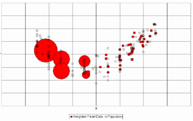
principle is visualized in figure 2.1. Early discussion on the strengths and weak-nesses of direct weighting by inverse estimated propensity scores can be found in Little (1986) and Little and Rubin (1987, p.58). See Tan (2006) for a likelihood formulation.

Assuming ˆπk(x) are consistently estimated consider now the the potential bias

of the π−weighted estimator. Let P r(Sk = 1|x, y) = πk(x, y) and denote

the joint density (X, Y) in the population by f(x, y), while in the sample by

f(x, y|s) = πk(x,y)f(x,y)

π(·,·) where π(·,·) =

R R

π(x, y)f(x, y)dydx is the average se-lection probability. Also let Cov(·) denote covariance, σ(·|x) the conditional standard deviation and ρ(·|x) the conditional correlation coefficient. By noting that R R π(x)−1π(x, y)f(x, y)dydx= 1 then the potential bias of ˆy_π is

B(Yˆπ) = E

P

s0SkYk/πk(x)

P

s0Skπk(x)−1

−E(Y)

≈

Z Z

y

π(y,x)

π(x) −1

f(y,x)dydx

= Cov

Y,π(Y,X) π(X)

=

Z

σ(Y|x)σ{π(x, Y)|x}

π(x) ρ{Y, π(x, Y)|x}

f(x)dx (2.17)

where the approximation is of order o(n−1).

Under correct specification π(y,x) = π(x) and the bias is exactly zero. Other-wise, the magnitude of B(Yˆπ) will depend both on the level of departure from

the π−model and distributional properties of f(y|x) and p(s|x). Specifically, bias will be small if at least one of the factors is small

(i) the conditional standard deviation of Y σ(Y|x) is small for all x , which happens if Y ≈E(Y|x) - that is the Y values are predicted well by the X, or

(ii)π(x, y) varies little withyfor fixedxwhich happens if at least approximately,

p(s|x, y)≈ p(s|x) for all x and y, which happens in a good prediction model of

(36)

[image:36.595.139.478.75.288.2]

Figure 2.1: The π-estimator: π− estimation recovers the joint distribution of (X, Y) by attaching weight∝π(x)−1to each point in{(Xk, Yk) :Sk= 1}but is sensitive to cases where

π≈0.

(iii) the conditional correlation ρ{Y, π(x,Y)|x} is close to zero for all x.

The main objection to Yˆπ is its sensitivity to the common support assumption.

Direct weighting can be highly unstable as respondents with very low values of

π are sharply adjusted - an idea visualized in figure 2.1 as well. This sensitivity can be seen both in the potential bias (2.17) which is a function ofπ−1 _{and in the}

expected variance; for example the selection-model variance of the π−estimator with known selection probabilities is V(Yˆπ|y) =P_s∈Sp(s)(

ˆ

Yπ−E(Yˆπ))2 which

under Poisson selection is

V(Yˆπ)≈N−2

X

k∈U

π_k−1−1(yk−y)2 (2.18)

which also is inflated in regions where π(x)≈0.

At the extremes when there is complete separation in the distribution f(x) be-tween s and s the estimator breaks down and is not defined. An interesting counterargument to this criticism (Tan, 2007) puts that this instability in fact properly reflects the separation in f(x) and thus the lack of information on y_s0

(37)

observed over the entire finite population. This is in contrast to m−estimation which is fitted over (Ys,Xs) , a major weakness I discuss in the following section.

In practice after choosing the π−weighted estimator, we must decide (i) the covariate set X to include in the π−model and (ii) the relevant model fit-ting/goodness of fit tests.

As for covariate selection, the fundamental recommendation, supported by the potential bias (2.17) is to include all covariates associated either to Y or S . This is echoed in advice such as in Rubin and Thomas (1996) and Heckman et al. (1998) who argue that there is no distinction between highly predictive covariates and weakly predictive ones in the performance of propensity score ad-justment and suggest including all observable covariates. Drake (1993) finds that misspecifications of the propensity score in terms of functional form have much smaller biases than similar misspecifications in m−model estimation. Millimet and Tchernis (2009) report a simulation that focuses on, essentially, the func-tional form of the propensity score and conclude that the penalty for overfitting is minimal. More recently Rubin (2009, p.1421) reiterates by stating that not controlling for an observed covariate is bad practical advice in all but the most unusual circumstances.

On the other hand, work on the effects of including covariates (into the propen-sity model) that have only weak or no effect on either the selection or outcome variables has been published countering the above consensus. For example in a simulation study Augurzky and Schmidt (2001) include a set of variables Xs_,

which strongly influence S, but do not or only weakly determineY and a second set Xy, that influence Y, but are irrelevant to S. Their result indicates that including both sets of covariates results in an increase in the MSE and recom-mend including only highly significant variables in the propensity score equation. Similarly, Brookhart et al. (2006) find that one should include covariates that are thought to be related to Y, whether or not they are related to the selection, while the opposite of including covariates only related toSincreases the variance of and estimator without decreasing its bias. Clarke (2005, 2009); Clarke et al. (2011) persuasively demonstrates that, for a misspecified model, the inclusion of additional control variables, which influence both S and Y increases the estima-tion bias dramatically.

(38)

its inclusion in the model, then the square of the variable and interactions with other variables can be tried. Ho et al. (2007) put this idea as the propensity score tautology ’: The estimated propensity score is a balancing score when we have a consistent estimate of the true propensity score; We know we have a con-sistent estimate of the score when matching on the propensity score balances the raw covariate. More recent balancing tests include testing for mean differences