Dimensional Effects on Densities of States and Interactions in Nanostructures

(1)

N A N O E X P R E S S

Dimensional Effects on Densities of States and Interactions

in Nanostructures

Rainer Dick

Received: 15 April 2010 / Accepted: 7 June 2010 / Published online: 2 July 2010 ÓThe Author(s) 2010. This article is published with open access at Springerlink.com

Abstract We consider electrons in the presence of

interfaces with different effective electron mass, and electromagnetic fields in the presence of a high-permit-tivity interface in bulk material. The equations of motion for these dimensionally hybrid systems yield analytic expressions for Green’s functions and electromagnetic potentials that interpolate between the two-dimensional logarithmic potential at short distance, and the three-dimensionalr-1potential at large distance. This also yields results for electron densities of states which interpolate between the well-known two-dimensional and three-dimensional formulas. The transition length scales for interfaces of thicknessLare found to be of order Lm/2m* for an interface in which electrons move with effective mass m*, and L=2 for a dielectric thin film with per-mittivity in a bulk of permittivity. We can easily test the merits of the formalism by comparing the calculated electromagnetic potential with the infinite series solutions from image charges. This confirms that the dimensionally hybrid models are excellent approximations for distances

rZL/2.

Keywords Density of states

Coulomb and exchange interactions in nanostructures Dielectric thin films

Introduction

When we suppress motion of particles in certain directions through confining potentials, e.g. in quantum wells or quantum wires, we often model the residual low energy excitations in the system through low-dimensional quan-tum mechanical systems. Prominent examples of this concern layered heterostructures, and one instance where the number d of spatial dimensions enters in a manner which is of direct relevance to technology is in the density of states. In the standard parabolic band approximation, this takes the form (with two helicity or spin states)

.ðdÞðEÞ ¼2HðEÞ

ffiffiffiffiffiffi

m

2p

r d ffiffiffiffi

E

p d2

Cðd=2Þhd: ð1Þ

These are densities of states perd-dimensional volume and per unit of energy. The corresponding dependence of the relation between the Fermi energy and the density n of electrons ond is

n_ðdÞ¼

2

hdCððdþ2Þ=2Þ

ffiffiffiffiffiffiffiffiffi

mEF 2p

r d

: ð2Þ

Variants of these equations (including summation over subbands) are often used for d=2 or d=1 to estimate carrier densities in quasi two-dimensional systems or nanowires, and the density of states plays a crucial role in all transport and optical properties of materials. Indeed, the obvious relevance for electrical conductivity properties in micro and nanotechnology implies that densities of states for d=1, 2, or 3 are now commonly discussed in engineering textbooks, but there is another reason why I anticipate that variants of Eq. (1) will become ever more prominent in the technical literature. Densities also play a huge role in data storage, but with us still relying on binary R. Dick (&)

Physics & Engineering Physics, University of Saskatchewan, 116 Science Place, Saskatoon, SK S7N 5E2, Canada e-mail: [email protected]

(2)

logic switching between two stable states (spin up or down, charge or no charge, conductivity or no conductivity), data storage densities are limited by the physical densities of the systems which provide the dual states. We could (and likely will) drive information technology and integration much further if we can find ways to utilize more than just two states of a physical system to store and process information. Then, data storage densities should become proportional to energy integrals R_DEdE.ðEÞ of local densities of states. Equation (1) for d=1 or d =2 is certainly applicable for particles which have low energies compared to the confinement energy of a nanowire or a quantum well, but how can we effectively model particles which are weakly confined to a nanowire or quantum well, or which are otherwise affected by the presence of a low-dimensional substructure? In these cases, we can devise dimensionally hybrid models [1, 2] which yield e.g. densities of states which interpolate between d =2 and

d=3 [3,4]. This construction will be reviewed in Sect.2. Based on the experience gained with dimensionally hybrid Hamiltonians for massive particles, we can also construct inter-dimensional Hamiltonians for photons which should be applicable to photons in the presence of high-permittivity thin films or interfaces. These models can also be solved in terms of infinite series expansions using image charges, and the merits of this approach can easily be tested. The case of high-permittivity thin films and testing the theory against image charge solutions will be discussed in Sect.3.

Dimensionally Hybrid Hamiltonians and Green’s Functions for Massive Particles in the Presence of Thin Films or Interfaces

We use the connection between Green’s functions and the density of states to generalize Eq. (1) for massive particles in the presence of a thin film or interface.

The energy-dependent Green’s function for a Hamilto-nianHwith spectrumEnand eigenstates |n,miis

GðEÞ ¼ 2m

h2GðEÞ ¼

1

EHþi¼

X Z

n;m

jn;mihn;mj

EEnþi ¼ PX Z

n;m

jn;mihn;mj

EEn

ipX Z

n;m

dðEEnÞjn;mihn;mj: ð3Þ

Here,mis a degeneracy index and the notation implies that continuous components in the indices (n,m) are integrated. The first equation simply states the relation between the resolvent GðEÞ of the Hamiltonian and the Green’s

function G(E) which is normalized as limm?0,E?0

G(E)|d=3=(4pr)-1.

The zero-energy Green’s function G(0) determines e.g. 2-particle correlation functions and electromagnetic inter-action potentials, and the energy-dependent Green’s func-tion G(E) determines e.g. scattering amplitudes for particles of energy E. Application for resistivity calcula-tions is therefore another technologically relevant appli-cation of Green’s functions. However, in the present section we are interested in this function because it also determines the local density of states in a system with HamiltonianHthrough the relation

.ðEn;~xÞ ¼2

X Z

m

h~xjn;mihn;mj~xi ¼ 4m

ph2=h~xjGðEnÞj~xi:

ð4Þ

Here, we explicitly included a factor 2 for the number of spin or helicity states, because the summation over degeneracy indices in (3,4) usually only involves orbital indices.

For our present investigation, the distinctive feature of the interface is that the particles move in it with an effective massm*, while their mass in the surrounding bulk is m. We use coordinates x¼ fx;yg parallel to a plane interface, which is located atz=z0. Bold vector notation is used for quantities parallel to the interface, e.g. ~p¼

p;pz

f gandr~¼ f$;ozg.

We assume that the interface has a thickness L. If the wavenumber component orthogonal to the interface is small compared to the inverse width, |k\L|1, i.e. if the de Broglie wavelength and the incidence angle satisfy

k 2pL|cos0|, we can approximate the kinetic energy of the particles through a second quantized Hamiltonian

H¼

Z

d2x

Z

dzh 2

2mr

~_wþ_ð_x_;_z_{Þ r}_~ wðx;zÞ

þ

Z

d2xh 2

2l$w þ

ðx;z0Þ $wðx;z0Þ; ð5Þ

wherel=m*/L. The corresponding first quantized Hamiltonian is

H¼p

2_þ_p2

z

2m þ jz0ihz0j p2

2l: ð6Þ

(3)

we will use a parabolic band approximation in the bulk and in the interface.

The energy-dependent Green’s function h~xjGðEÞj~x0i hzjGðE;xx0Þjz0idescribes scattering effects in the pres-ence of the interface but also applies to scattering off perturbations which are not located on the interface. In an axially symmetric mixed representation

hk;zjGðEÞjk0;z0i ¼ hzjGðE;kÞjz0idðkk0Þ ð7Þ

the first order approximation to scattering of an orthogonally incoming plane wave off an impurity potential

Vðx;zÞ ¼ 1 4p2

Z

d2kVðk;zÞexpðikxÞ corresponds to

wðx;zÞ ¼ _{ffiffiffiffiffiffi}1 2p

p 3 expðik?zÞ m

2p2_h2

Z

d2x0

Z

d2k

Z

dz0hzjGðE;kÞjz0iVðx0;z0Þ

exp½iðkxþk?z0Þ expðikx0Þ

¼ _{ffiffiffiffiffiffi}1 2p

p 3 expðik?zÞ m

2p2_h2

Z

d2k

Z

dz0hzjGðE;kÞjz0iVðk;z0Þexp½iðkxþk?z0Þ

:

Green’s functions for surfaces or interfaces are commonly parametrized in an axially symmetric mixed representation like GðE;k;z;z0Þ. In bra-ket notation, this corresponds for the free Green’s functionG0(E), which is also translation invariant inzdirection, to

hk;zjG0ðEÞjk0;z0i ¼G0ðE;k;zz0Þdðkk0Þ:

We will briefly recall the explicit form of the free Green’s function G0(E) in the axially symmetric mixed parametrization for later comparison. The equation

o2_zk2þ2mE

h2

G0ðE;k;zÞ ¼ dðzÞ

yields

G0ðE;k;zÞ ¼

1 2p

Z

dk?

expðik?zÞ k2

?þk

2_ð2_mE=_h2_Þ_i

¼hHðh

2_k2

2mEÞ 2 ffiffiffiffiffiffiffiffiffiffiffiffiffiffiffiffiffiffiffiffiffiffiffiffih2k22mE

p exp pffiffiffiffiffiffiffiffiffiffiffiffiffiffiffiffiffiffiffiffiffiffiffiffih2k22mEjzj

h

þihHð2mEh

2_k2_Þ

2pffiffiffiffiffiffiffiffiffiffiffiffiffiffiffiffiffiffiffiffiffiffiffiffi2mEh2k2

exp ipffiffiffiffiffiffiffiffiffiffiffiffiffiffiffiffiffiffiffiffiffiffiffiffi2mEh2k2jzj

h

:

ð8Þ

To study how this is modified in the presence of the interface, we observe that the Hamiltonians (5) or (6) yield a Schro¨dinger equation

Ewðx;zÞ ¼ h

2

2mDwðx;zÞ

h2

2ldðzz0Þ$

2_w_ð_x_;_z_Þ_:

The corresponding equation for the Green’s function or 2-point correlation function is

2m

h2EþDþdðzz0Þ m l$

2

hx;zjGðEÞjx0;z0i

¼ dðxx0Þdðzz0Þ: ð9Þ

The solution of this equation is described in the Appendix. In particular, we find the representation (see Eq. (27))

hzjGðE;kÞjz0i ¼

hHðh2k22mEÞ 2 ffiffiffiffiffiffiffiffiffiffiffiffiffiffiffiffiffiffiffiffiffiffiffiffih2k22mE

p exp pffiffiffiffiffiffiffiffiffiffiffiffiffiffiffiffiffiffiffiffiffiffiffiffih2k22mEjzz 0_j

h

hk

2_‘

ffiffiffiffiffiffiffiffiffiffiffiffiffiffiffiffiffiffiffiffiffiffiffiffi

h2k22mE

p

þhk2‘

exp pffiffiffiffiffiffiffiffiffiffiffiffiffiffiffiffiffiffiffiffiffiffiffiffih2k22mEjzz0j þ jz 0_z

0j

h

þihHð2mEh

2_k2_Þ

exp ipffiffiffiffiffiffiffiffiffiffiffiffiffiffiffiffiffiffiffiffiffiffiffiffi2mEh2k2jzz

0_j

h

i hk

2_‘

2mEh2k2

p

þihk2‘

exp ipffiffiffiffiffiffiffiffiffiffiffiffiffiffiffiffiffiffiffiffiffiffiffiffi2mEh2k2jzz0j þ jz

0_z

0j

h

; ð10Þ

where the definition ‘:m/2l =Lm/2m* was used. The

‘-independent terms in (10) correspond to the free Green’s functionG0(E) (8).

The interface at z0 breaks translational invariance in z direction, and we have with Eq. (7)

.ðE;zÞ ¼ 4m

ph2=hx;zjGðEÞjx;zi

¼ m

p3_h2=

Z

d2khzjGðE;kÞjzi:

We will use the result (10) to calculate the density of states .ðE;z0Þin the interface. Substitution yields

.ðE;z0Þ ¼ m p3_h2=

Z

d2khz0jGðE;kÞjz0i

¼ m

p2_hHðEÞ

Z ffiffiffiffiffiffiffip2mE=h

0

dkk

2mEh2k2

p

2mEh2k2_þ_h2_k4_‘2;

(4)

.ðE;z0Þ ¼ mHðEÞ

2p2_h2_‘p_hffiffiffiffiffiffiffiffiffiffiffiffiffiffiffiffiffiffiffiffiffiffiffi2₈_mE‘2Hðh

2₈_mE‘2_Þ

2harctan ‘

8mE

p

hþpffiffiffiffiffiffiffiffiffiffiffiffiffiffiffiffiffiffiffiffiffiffiffih28mE‘2

p 2 h

ffiffiffiffiffiffiffiffiffiffiffiffiffiffiffiffiffiffiffiffiffiffiffi

h28mE‘2

p

þmHð8mE‘

2_h2_Þ

2p2_h2_‘

_{ffiffiffiffiffiffiffiffiffiffiffiffiffiffiffiffiffiffiffiffiffiffiffi}h 8mE‘2_h2

p ln ‘

8mE

p

pffiffiffiffiffiffiffiffiffiffiffiffiffiffiffiffiffiffiffiffiffiffiffi8mE‘2_h2

h

!

þp 2

" #

:

ð11Þ

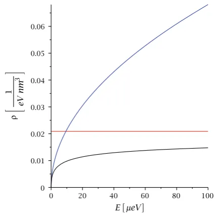
This is a more complicated result than the density (1) for

d=2 or d=3. However, it reduces to either the two-dimensional or three-two-dimensional density of states in the appropriate limits, see Fig.1. For large energies, i.e. if the states only probe length scales smaller than the transition length scale ‘, we find the two-dimensional density of states properly rescaled by a dimensional factor to reflect that it is a density of states per three-dimensional volume, 8mE‘2 h2: .ðE;z0Þ !HðEÞ

m

4ph2‘¼

1

4‘.ðd¼2ÞðEÞ:

ð12Þ For small energies, i.e. if the states probe length scales larger than‘, we find the three-dimensional density of states 8mE‘2 h2: .ðE;z0Þ !HðEÞ

ffiffiffiffiffiffiffiffi

2m3

p

p2_h3

ffiffiffiffi

E

p

¼._ð_d_¼₃_ÞðEÞ:

ð13Þ

This limiting behavior for interpolation between two and three dimensions is consistent with what is also observed for the zero-energy Green’s function in the interface, see equations (21–22) below.

Equation (11) also implies interpolating behavior for the relation between electron density and Fermi energy on the interface. The full relation is

nðz0Þ ¼

mEF p

ffiffiffi

8 p

p2_h‘2

1 16p‘3þ

Hðh28mEF‘2Þ 8p2_h2_‘3

p 2 4mEF‘

2_þ_h ffiffiffiffiffiffiffiffiffiffiffiffiffiffiffiffiffiffiffiffiffiffiffiffiffiffi_h2₈_mE

F‘2

q

2h

ffiffiffiffiffiffiffiffiffiffiffiffiffiffiffiffiffiffiffiffiffiffiffiffiffiffi

h28mEF‘2

q

arctan

ffiffiffiffiffiffiffiffiffiffiffiffi

8mEF p

‘

hþ ffiffiffiffiffiffiffiffiffiffiffiffiffiffiffiffiffiffiffiffiffiffiffiffiffiffih28mEF‘2

p

!#

þHð8mEF‘

2_h2_Þ

8p2_h‘3

" ffiffiffiffiffiffiffiffiffiffiffiffiffiffiffiffiffiffiffiffiffiffiffiffiffiffi

8mEF‘2h2

q

ln

8mEF p

‘ ffiffiffiffiffiffiffiffiffiffiffiffiffiffiffiffiffiffiffiffiffiffiffiffiffiffi8mEF‘2h2

p

h

!

þ2pmEF‘

2

h

#

:

This approximates two-dimensional behavior for

mEF‘2h2,

nðz0Þ ’ mEF

4ph2‘¼

1 4‘nðd¼2Þ;

and three-dimensional behavior formEF‘2h2,

nðz0Þ ’

2mEF

p 3

3p2_h3 ¼nðd¼3Þ:

It is intuitively understandable that the presence of a layer reduces the available density of states for given energy, or equivalently increases the Fermi energy for a given density of electrons. The presence of a layer generically implies boundary or matching conditions which reduce the number of available states at a given energy.

A condition for relevance of the inter-dimensional behavior is a large transition scale compared to the layer thickness, ‘L, see also Fig.2. In terms of effective particle mass, this means

mm; ð14Þ

i.e. the energy band in the interface should be more strongly curved than in the bulk matrix for the transition to two-dimensional behavior to be observable.

Electric Fields in the Presence of High-Permittivity Thin Films or Interfaces

[image:4.595.317.530.55.266.2]

(5)

interactions through the electrostatic potential UðrÞ ¼

qGðrÞ=. Here, q is an electric charge in a dielectric material of permittivity. The zero-energy Green’s func-tion indspatial dimensions is given by

GðrÞ ¼

r=2; d¼1;

ð2pÞ1lnðr=aÞ; d¼2; C d2

2

4pffiffiffipdrd2

1

; d3:

8 > < >

: ð15Þ

We cannot infer from the previous section that the zero energy limit of the inter-dimensional Green’s function calculated there also yields a dimensionally hybrid potential, because we were dealing with solutions of Schro¨dinger’s equation instead of the Gauss law. However, we can rederive the zero energy limit of that Green’s function from the Gauss law for electromagnetic fields in the presence of a high-permittivity interface.

Suppose we have charge carriers of chargeqand massm

in the presence of an interface with permittivity and permeabilityl*, We continue to denote vectors parallel to the interface in bold face notation, ~x¼ fx;zg, r

~_{¼ f}_$_;_o_z_g_;~_A_{¼ f}_A_;_A_z_{g, etc.}

If the photon wavelengths and incidence angles satisfy the condition k 2pL|cos0|, we can approximate the system with an action

S¼L

Z

d2x

2E

~2 1

2l B ~2

z¼z0

þ

Z

d3~x ih

2 w þo

otw

o otw

þ w

qwþUwþqh 2mw

þ_~_r_~_B_w_þ 1 2m ihr

~_wþ_qwþ_~_A

ihr~wþqA~wþ 2E

~2 1

2lB ~2

:

Variation with respect to the electrostatic potential,

dS=dU¼0, yields the Gauss law in the form

r~E~þLdðzz0Þ$E¼qwþw ð16Þ

and the continuity conditionEz(z0-0)=Ez(z0?0). We solve Eq. (16) in Coulomb gauge,

Uð~;x tÞ ¼q

Z

d3~x0Gð~;x~x0Þwþð~x0;tÞwð~x0;tÞ ð17Þ where the Green’s function has to satisfy

DGð~;x~x0Þ þL

dðzz0Þ$ 2_G_ð_x

~;~x0Þ ¼ dð~x~x0Þ: ð18Þ

This equation is the zero energy limit of Eq. (9) with the substitution

m

l L

m m

!L :

We can therefore read off the solution from the results of the previous section withE =0 and now‘L=2.

Equation (10) yields in particular hzjGðkÞjz0i ¼

1

2k expðkjzz

0_jÞk‘expðkjzz0j kjz0z0jÞ

1þk‘

with k jkj. Fourier transformation yields hzjGðxÞjz0i ¼

Z 1

0 dk

Z 2p

0

duexpðikjxjcosuÞ

8p2

expðkjzz0jÞ

k‘expðkjzz0j kjz 0_z

0jÞ

1þk‘

¼

Z 1

0 dk 4p

expðkjzz0jÞ

k‘expðkjzz0j kjz 0_z

0jÞ

1þk‘

J0ðkjxjÞ:

ð19Þ

The zero-energy Green’s function in the interface is given in terms of a Struve function and a Neumann function1,

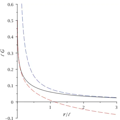
Fig. 2 The upper dotted (blue) lineis the three-dimensional Green’s function (4pr)-1in units of‘-1_{, the continuous line is the Green’s}

function (19) in units of‘-1_{, and the}_{lower dotted (red) line} _{is the}

two-dimensional logarithmic Green’s function ‘G= -(c?ln(r/ 2‘))/(4p)

1 _{Our notations for special functions follow the conventions of}

[image:5.595.70.274.54.258.2]

(6)

GðrÞ ¼ hz0jGðr¼ jxx0jÞjz0i ¼

Z 1

0

dk 4p

J0ðkrÞ

1þk‘

¼ 1 8‘ H0

r ‘ Y0

r ‘

h i

: ð20Þ

This yields logarithmic behavior of interaction potentials at small distancesr‘and 1/rbehavior for large separation

r‘of charges in high-permittivity thin films,

r‘: GðrÞ ¼ 1

4p‘ cln r

2‘ þ r ‘þ O

r2 ‘2

;

ð21Þ

r‘: GðrÞ ¼ 1 4pr 1

‘2 r2þ O

‘4 r4

; ð22Þ

see also Fig.2.

For the comparison with image charges, we setz0=0 and recall that the solution for the potential of a chargeqat

x¼0,z=0 proceeds through theansatz

jzjL=2: U¼ 1 4p

"

q

ffiffiffiffiffiffiffiffiffiffiffiffiffi

r2_þ_z2

p :

þX 1

n¼1 qn

1

r2_þð_z_nL_Þ2

q þ _{ffiffiffiffiffiffiffiffiffiffiffiffiffiffiffiffiffiffiffiffiffiffiffiffiffiffi}1

r2_þð_z_þ_nL_Þ2

q 0 B @ 1 C A 3 7 5 ¼ X 1 n¼1

qjnj

4p

r2_þð_z_nL_Þ2

q ;

z[L=2: U¼ 1 4p

Q

ffiffiffiffiffiffiffiffiffiffiffiffiffi

r2_þ_z2

p þX

1

n¼1

Qn

r2_þð_z_þ_nL_Þ2

q 0 B @ 1 C A ¼X 1

n¼0

Qn

4p

r2_þð_z_þ_nL_Þ2

q ;

and symmetric continuation toz\-L/2. This yields electric fields

jzj L=2: Er¼

X1

n¼1

qjnjr

4p

ffiffiffiffiffiffiffiffiffiffiffiffiffiffiffiffiffiffiffiffiffiffiffiffiffiffiffiffiffi

r2_{þ ð}_z_nL_Þ2

q 3;

Ez¼

X1

n¼1

qjnjðznLÞ

4p

r2_{þ ð}_z_nL_Þ2

q 3;

z[L=2: Er¼

X1

n¼0

Qnr

4p

r2_{þ ð}_z_þ_nL_Þ2

q 3;

Ez¼

X1

n¼0

QnðzþnLÞ

4p

q 3;

and the junction conditions atz=L/2 yield fornC0 from the continuity ofEr,

qnþqnþ1

¼Qn

;

and from the continuity ofDz,

qnqnþ1¼Qn:

These conditions can be solved through

qn¼

þ

n

q; Qn¼ 2 þ þ n q;

jzj L=2: U¼ q 4p

X1

n¼1

þ

jnj

1

ffiffiffiffiffiffiffiffiffiffiffiffiffiffiffiffiffiffiffiffiffiffiffiffiffiffiffiffi

r2_{þ ð}_z_nL_Þ2

q ;

z[L=2: U¼ q

2pðþÞ

X1

n¼0

þ

n

1

ffiffiffiffiffiffiffiffiffiffiffiffiffiffiffiffiffiffiffiffiffiffiffiffiffiffiffiffi

q :

In particular, the potential atz=0 is UðrÞ ¼ q

4pr þ q

2p

X1

n¼1

þ

n

1

ffiffiffiffiffiffiffiffiffiffiffiffiffiffiffiffiffiffiffi

r2_þ_n2_L2

p : ð23Þ

We have

X1

n¼1

þ

n

¼ 2

and therefore for [ q

4pr

\UðrÞ UðrÞa¼0¼ q

4pr:

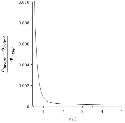
The solution from image charges is in very good agreement with the analytic model for distances rZL/2, where both the image charge solution and the analytic model show strong deviations from the bulkr-1behavior. This is illustrated in Fig.3 by plotting the reduced electrostatic potential for a charge q, LUðrÞ=q¼LGðrÞ in the interface.

It is also instructive to plot the relative deviation

ðUimageUhybridÞ=Uimage between the dimensionally

hybrid potential UhybridðrÞ ¼qGðrÞ= which follows from (20) and the potentialUimage(23) from image charges.

Figure4 shows that for rZL/2, the dimensionally hybrid model is a very good approximation to the potential from image charges with accuracy better than 10-2 if

=¼100. For=¼10, the accuracy is still better than 4 910-2.

Summary

(7)

two-dimensional behavior and three-two-dimensional behavior. The analytic model for the electromagnetic fields is in very good agreement with the infinite series solution already for small distance scalesrZL/2, where the potential strongly deviates from the standard bulkr-1potential. At distance scales smaller thanL/2, r-1, behavior seems to dominate again for the electrostatic potential, in agreement with expectations that for distances which are small compared to

the lateral extension of a dielectric slab, bulk behavior should be restored. However, note that neither the inter-dimensional analytic model nor the solution from image charges is trustworthy for very small distances, because both models rely on a continuum approximation through the use of effective permittivities, but the continuum approximation should break down at sub-nanometer scales. The most important finding is that interfaces and thin films of width L should exhibit transitions between two-dimensional and three-two-dimensional distance laws for physical quantities at length scales of order Lm/2m* or

L=2, respectively. Interfaces with strong band curvature or high permittivity should provide good samples for experimental study of the transition between two-dimen-sional and three-dimentwo-dimen-sional behavior.

Acknowledgements This research was supported by NSERC Canada.

Open Access This article is distributed under the terms of the Creative Commons Attribution Noncommercial License which per-mits any noncommercial use, distribution, and reproduction in any medium, provided the original author(s) and source are credited.

Appendix: Solution of Eq. (9)

Substitution of the Fourier transform hx;zjGðEÞjx0;z0i

¼ 1 4p2

Z

d2k

Z

d2k0hk;zjGðEÞjk0;z0iexp½iðkxk0x0Þ

into Eq. (9) yields 2m

h2Ek 2

þo2_z

hk;zjGðEÞjk0;z0i

m

lk 2

dðzz0Þhk;zjGðEÞjk0;z0i

¼ dðkk0Þdðzz0Þ: ð24Þ

This yields with (7) the condition 2m

h2Ek 2

þo2_z

hzjGðE;kÞjz0i

m

lk 2

dðzz0ÞhzjGðE;kÞjz0i

¼ dðzz0Þ:

Fourier transformation with respect to zyields 2m

h2Ek 2_k2

?

hk?jGðE;kÞjz0i

m

2plk 2Z _d

j?exp½iðj?k?Þz0 hj?jGðE;kÞjz0i ¼ 1ffiffiffiffiffiffi

2p

p expðik?z0Þ: ð25Þ

This result implies thathk?jGðE;kÞjz0ihas the form Fig. 3 Different reduced electrostatic potentials are plotted for

=¼100. The upper dotted (green) lineis the three-dimensional reduced potential L/(4pr). The central dotted (blue) line is the reduced potential following from the image charge solution (22). The solid (black) lineis the potential from the analytic model (19). The lower dotted (red) line is the reduced logarithmic potential. The reduced potentials from our analytic model and from image charges are indistinguishable forr[rsimL=2, see also Fig.4

[image:7.595.68.270.56.254.2] [image:7.595.63.279.358.570.2]

(8)

expðik?z0Þhk?jGðE;kÞjz0i ¼ ðexp½ik?ðz0z0Þ =

ffiffiffiffiffiffi

2p

p

Þ þfðE;k;z0Þ

k2

?þk

2_ð2_mE=_h2_Þ

with the yet to be determined functionfðE;k;z0Þsatisfying

fðE;k;z0Þ

þ m 2plk

2Z _d j?

ðexp½ij?ðz0z0Þ =

ffiffiffiffiffiffi

2p

p

Þ þfðE;k;z0Þ

j2

?þk2 ð2mE=h2Þ ¼0:

For the treatment of the integrals, we should be consistent with the calculation of the free retarded Green’s function (8),

Z _d_j

? 2p

exp iðj?zÞ j2

?þk

2_ð2_mE=_h2_Þ_i

¼h 2Hðh

2_k2₂_mE_Þexp

h2k22mE

p

jzj=h

h2k22mE

p

þih

2Hð2mEh

2_k2_Þexp i

2mEh2k2

p

jzj=h

2mEh2k2

p :

This yields 1þmh

2lk 2 Hðh

2_k2

2mEÞ

h2k22mE

p þiHð2mEh

2_k2

Þ

2mEh2k2

p

fðE;k;z0Þ ¼ mh 2lpffiffiffiffiffiffi2pk

2 Hðh

2_k2₂_mE_Þ

h2k22mE

p

exp pffiffiffiffiffiffiffiffiffiffiffiffiffiffiffiffiffiffiffiffiffiffiffiffih2k22mEjz 0_z

0j

h

:

þiHð2mEh

2_k2

Þ

2mEh2k2

p exp ipffiffiffiffiffiffiffiffiffiffiffiffiffiffiffiffiffiffiffiffiffiffiffiffi2mEh2k2jz

0_z

0j h ; and therefore

hk?jGðE;kÞjz0i ¼ 1

ffiffiffiffiffiffi 2p

p 1

k2

?þk2 ð2mE=h2Þ i ½expðik?z0Þ

hk 2

‘Hðh2_k2 2mEÞ ffiffiffiffiffiffiffiffiffiffiffiffiffiffiffiffiffiffiffiffiffiffiffiffi

h2k22mE p

þhk2‘

exp ik?z0

h2k2

2mE

p _jz0_z

0j

h

ihk 2

‘Hð2mEh2k2_Þ ffiffiffiffiffiffiffiffiffiffiffiffiffiffiffiffiffiffiffiffiffiffiffiffi 2mEh2_k2 p

þihk2‘

exp ik?z0þi

ffiffiffiffiffiffiffiffiffiffiffiffiffiffiffiffiffiffiffiffiffiffiffiffi 2mEh2k2

p _j_z0_z

0j h ; ð26Þ

where the definition‘:m/2l =Lm/2m*was used. Fourier transformation of Eq. (26) with respect tok\yields finally

hzjGðE;kÞjz0i ¼

hHðh2k22mEÞ 2pffiffiffiffiffiffiffiffiffiffiffiffiffiffiffiffiffiffiffiffiffiffiffiffih2k22mE

exp pffiffiffiffiffiffiffiffiffiffiffiffiffiffiffiffiffiffiffiffiffiffiffiffih2k22mEjzz 0_j h hk 2 ‘ ffiffiffiffiffiffiffiffiffiffiffiffiffiffiffiffiffiffiffiffiffiffiffiffi

h2k22mE

p

þhk2‘

exp pffiffiffiffiffiffiffiffiffiffiffiffiffiffiffiffiffiffiffiffiffiffiffiffih2k22mEjzz0j þ jz 0_z

0j

h

þihHð2mEh

2_k2_Þ

exp ipffiffiffiffiffiffiffiffiffiffiffiffiffiffiffiffiffiffiffiffiffiffiffiffi2mEh2k2jzz

0_j

h

i hk

2_‘

2mEh2k2

p

þihk2‘

exp ipffiffiffiffiffiffiffiffiffiffiffiffiffiffiffiffiffiffiffiffiffiffiffiffi2mEh2k2jzz0j þ jz

0_z

0j

h

: ð27Þ

The Green’s function with onlykspace variables hk;k?jGðEÞjk0;k0?i ¼ hk?jGðE;kÞjk?0 idðkk0Þ

is found from the Fourier transform of Eq. (25),

k2þk2_?2m

h2E

hk?jGðE;kÞjk0?i þ ‘ pk

2

Z

dj?exp½iðj? k?Þz0 hj?jGðE;kÞjk0?i

¼dðk?k?0Þ

and the ensuing equations expðik?z0Þhk?jGðE;kÞjk?0i ¼expðik?z0Þdðk?k

0

?Þ þfðE;k;k0?Þ k2

?þk

2_ð2_mE=_h2_Þ ;

fðE;k;k0_?Þ þk

2_‘

pfðE;k;k 0 ?Þ

Z _d_j

?

j2

?þk

2_ð2_mE=_h2_Þ

¼ k

2_‘

p

expðik0_?z0Þ k02

?þk

2

ð2mE=h2Þ:

This yields hk?jGðE;kÞjk

0

?i

¼ 1

k2

?þk

2_ð2_mE=_h2_Þ_i dðk?k 0 ?Þ h k 2_‘ p

exp½iðk0_?k?Þz0 k02

?þk

2

ð2mE=h2Þ i

h2k22mE

p

Hðh2k22mEÞ

h2k22mE

p

þhk2‘

þ

2mEh2k2

p

Hð2mEh2k2Þ

2mEh2k2

p

þihk2‘

!#

:

(9)

References

1. R. Dick, Int. J. Theor. Phys.42, 569 (2003) 2. R. Dick, Nanoscale Res. Lett.3, 140 (2008) 3. R. Dick, Phys. E40, 524 (2008)

4. R. Dick, Phys. E40, 2973 (2008)

5. Y.A. Bychkov, E.I. Rashba, JETP Lett.39, 78 (1984) 6. Y.A. Bychkov, E.I. Rashba, J. Phys. C17, 6039 (1984) 7. E. Cappelluti, C. Grimaldi, F. Marsiglio, Phys. Rev. Lett. 98,

167002 (2007)

8. E. Cappelluti, C. Grimaldi, F. Marsiglio, Phys. Rev. B76, 085334 (2007)

9. B. Srisongmuang, P. Pairor, M. Berciu, Phys. Rev. B78, 155317 (2008)

10. P. Vasilopoulos, X.F. Wang, Phys. E40, 1729 (2008) 11. S.-S. Li, J.-B. Xia, Nanoscale Res. Lett.4, 178 (2009) 12. G.W. Semenoff, Phys. Rev. Lett.53, 2449 (1984)

13. V. Apalkov, X.F. Wang, T. Chakraborty, Int. J. Mod. Phys. B21, 1165 (2007)

14. L. Covaci, M. Berciu, Phys. Rev. Lett.100, 256405 (2008) 15. T. Li, Z. Zhang, Nanoscale Res. Lett.5, 169 (2010)