Robust 3D face landmark localization based on local coordinate coding

(1)

BIROn - Birkbeck Institutional Research Online

Song, M. and Tao, D. and Sun, S. and Chen, C. and Maybank, Stephen

J. (2014) Robust 3D face landmark localization based on local coordinate

coding. IEEE Transactions on Image Processing 23 (12), pp. 5108-5122.

ISSN 1057-7149.

Downloaded from:

Usage Guidelines:

Please refer to usage guidelines at

or alternatively

(2)

Robust 3D Face Landmark Localization based on

Local Coordinate Coding

Mingli Song,

Senior Member, IEEE,

Dacheng Tao,

Senior Member, IEEE,

Shengpeng Sun, Chun Chen, and

Stephen J. Maybank

Fellow, IEEE,

Abstract—In the 3D facial animation and synthesis community, input faces are usually required to be labeled by a set of landmarks for parameterization. Because of the variations in pose, expression and resolution, automatic 3D face landmark localization remains a challenge. In this paper, a novel landmark localization approach is presented. The approach is based on Local Coordinate Coding (LCC) and consists of two stages. In the first stage, we perform nose detection, relying on the fact that the nose shape is usually invariant under the variations in the pose, expression and resolution. Then, we use the Iterative Closest Points (ICP) algorithm to find a 3D affine transformation that aligns the input face to a reference face. In the second stage, we perform re-sampling to build correspondences between the input 3D face and the training faces. Then, an LCC-based localization algorithm is proposed to obtain the positions of the landmarks in the input face. Experimental results show that the proposed method is comparable to state of the art methods in terms of its robustness, flexibility and accuracy.

Index Terms—Landmark, 3D Affine Transformation, Face Alignment, Face Re-sampling, Iterative Closest Points, Local Coordinate Coding.

I. INTRODUCTION

T

HREE-dimensional (3D) faces have been widely used in many applications in computer vision, computer graphics and virtual reality. With the development of scanning tech-nology, large numbers of 3D coordinates can be obtained by 3D scanning devices, such as laser scanners, structured light scanners and other devices, in a very short time. Due to the limitation of the scanning devices, the 3D face data, which are usually in the form of point clouds, are acquired from different distances, orientations and expressions, which leads to enormous variations in the pose, face deformation, resolution, and even facial area. To build correspondences between the 3D faces that have different resolutions, poses, expressions and facial areas, many computer graphics and computer vision applications require corresponding landmarks for 3D face parameterization, which is the basis of further

Manuscript received January 18, 2013; revised August 5, 2014; accepted September 24, 2014. This work was supported in part by the National Natural Science Foundation of China under Grant 61170142, by the the Program of International S&T Cooperation (2013DFG12840), National High Technology Research and Development Program of China (2013AA040601), and by Australian Research Council Projects DP-140102164 and FT-130101457.

M. Song S. Sun, and C. Chen are with the College of Computer Science, Zhejiang University, Hangzhou 310027, China.

D. Tao is with the Centre for Quantum Computation & Intelligent Systems and the Faculty of Engineering and Information Technology, University of Technology, Sydney, 235 Jones Street, Ultimo, NSW 2007, Australia (email: [email protected]).

S. J. Maybank is with the Department of Computer Science and Information Systems, Birkbeck College, University of London

manipulation such as expressive analogy and animation. The landmarks are a set of 3D locations in a 3D face that are positioned to describe and parameterize the shape and semantics of the 3D faces.

Many 3D face applications [30], [44] locate the landmarks manually by using interactive tools, which is straightforward yet time consuming. Fortunately, a variety of methods for 3D face landmark localization have been proposed in recent years. These methods are divided into two groups: feature detection-based methods and statistical point distribution model (PDM)-based methods.

A. Feature Detection-based Approach

In the feature detection-based methods, the landmarks are defined by significant features, such as nose tip, nose wing, eye corners and mouth corners. These features are easily modeled by local descriptors. Lu et al. [1] proposed an algorithm to detect the nose tip on a rotated 3D face and to correct the facial pose by angle space quantization. However, this algorithm is based on the hypothesis that the nose tip on a frontal face is the closest point to the scanner. However, this hypothesis is not tenable in many cases. In addition, this method is computationally expensive when the angle space quantization is fine grained. Similar methods have been proposed by Perakis

et al.[3] to automatically detect the nose. In [3], the face pose is aligned by Procrustes analysis in which the candidate nose points are extracted based on the curvature information, and the mean shape is used to compute the rigid transformation. The candidate points that have a minimum Procrustes distance are regarded as nose points.

Many curvature-based methods have also been proposed to detect the nose tip [5]–[7]. The shape index [8] is used by Colbry et al. in which a statistical model is used to identify the nose position. Lin [6] uses principle curvatures and combines 2D and 3D data to describe the face. A search is conducted along the normal directions from the boundaries of the eyes to find the nose tip. Segundoet al. [7] proposed a method to detect the nose tip by combining traditional image segmentation techniques and an adapted method for 2D facial feature extraction with the curvature information. All of these nose detection methods produce good results for frontal faces but have limited capabilities for faces that are in arbitrary poses.

(3)

Only the points that correspond to the nose ridge should form a line in thex-yplane. However, this approach requires a near-frontal face. Dibeklio˘glu et al. [11] introduced a statistical method and a heuristic method for nose tip detection. The statistical method is based on an analysis of local features using the depth map and the gradient information of the depth map. The heuristic method locates the nose tip utilizing curvature values to address the pose variations. However, the statistical method cannot handle 3D faces that have pose variations, and the heuristic method is inaccurate on the 3D faces that have a yaw rotation that is greater than 45 degrees. Romero-Huertas et al.[12] used a graph model to locate the inner eye corners and the nose tip simultaneously. A graph matching algorithm is based on a distance-to-local plane node property and a Euclidean distance arc property. The feature combination that has the minimum Mahalanobis distance is selected. However, this method is sensitive to changes in the scale and radius of the distance-to-local plane.

Creusotet al.presented a multimodal feature point localiza-tion approach [14]. In [14], multiple local surface descriptors are used to extract interesting points of specific salient shapes first. Then, a model-fitting operation is exploited to select the facial feature points from the extracted interesting points. In the meantime, Fanelli et al.[15] developed a random forest-based facial feature detection system, in which a set of fixed-sized patches were extracted to vote for each of the salient feature points, e.g., eye corners, mouth corners and chin tip. The random forest-based facial feature point detection system can robustly and accurately locate the feature points on the 3D face sequence in real time.

It is noticeable that all of the above-mentioned methods align the face by relying on one vertex or a few reliable vertices, such as the nose tip and the eye corners. However, it is known that in many applications (e.g., face animation, parameterization, synthesis), the landmarks are required to be located at the forehead, cheeks, side of the face and other specific positions. It remains challenging to find reliable landmarks in those areas of the face that do not appear to have any significant features.

B. Statistical Point Distribution Model-based Approach

In 1995, Cootes and Taylor [13] proposed an Active Shape Model (ASM) to locate objects in images. Then, an Active Appearance Model (AAM) [17]–[23] was developed for face landmark detection. Recently, AAM has been extended to 3D face modeling [24]–[26]. Although these algorithms can detect a set of landmarks by fitting an AAM to an image, 2D image or 3D texture information is required. These algorithms are not suitable if the data consist of only a 3D point cloud or a triangulated face mesh.

Nair et al. [4] presented a 3D face landmark localization method that was based on a point distribution model (PDM). The PDM is a statistical model that describes the relative positions of the landmarks. The learned PDM is used to fit the 3D face using a transformation between the model points and the candidate vertices on the mesh. The landmarks defined in the PDM include not only the eye and mouth

corners and the nose and chin tips but also the eyebrows. However, the PDM is sensitive to variations in expression and to incomplete coverage of the 3D face. Afterward, Perakis et al. [10] introduced a 3D facial landmark localization method that was robust to yaw and expression changes. In [10], the shape index and spin image are used as features for detecting candidate landmarks e.g., eye corners, mouth corners, and nose tip. Then, a pre-trained PDM is explored to filter the landmarks.

To overcome the limitation of [15], Fanelli et al. further built a random forest based AAM (RF-AMM) [16] to locate more landmarks robustly, in which the random forest based pose estimation [15] is used to accomplish the initialization. RF-AAM achieves real-time performance and high accuracy against variations in expression and head pose. However, it is noticeable that both the random forest in [15] and the RF-AAM in [16] require that the testing data have a similar resolution to the training data.

In this paper, we propose a new framework for 3D face landmark localization that is based on local coordinate coding, which enables us to locate landmarks robustly under variations in pose, expression and resolution and even in cases when the 3D face is not completely covered by the data. Our approach consists of two stages. In the first stage, 3D face alignment is performed based on nose detection. Our nose detection is different from all of the methods mentioned above in that the whole nose region is detected including the bridge and the sides of the nose. After nose detection, we apply an affine transform to obtain a coarse alignment between the 3D face and a reference 3D face. Then, an ICP algorithm [2] is employed to refine the alignment. In the second stage, we first perform 3D face re-sampling to build the training database for LCC-based [27] landmark localization. Then, a coupled dictionary is learned based on the training database and the corresponding landmarks. Afterwards, given a new 3D face, a set of landmarks are synthesized based on the coupled dictionary. Finally, the landmarks are located under the guidance of synthesized landmarks that are based on the coupled dictionary.

The remainder of this paper is organized as follows. Sec-tion II describes the 3D face alignment that is based on nose detection. Section III describes the 3D face landmark localization that is based on LCC. Section IV presents the ex-perimental results. Finally, Section V summarizes our method and proposes future directions for further research.

II. STAGEONE: COARSEALIGNMENT

(4)

(a) (b) (c)

3D Face with Normals

Left Side Right Side

[image:4.612.313.567.283.496.2]

Front View Section View

Fig. 1. (a) 3D Face with normals. (b) Front view of the nose with normals. (c) Section view of the nose with normals.

of the face, and it is easy to detect. Third, the nose is the most stable feature of the face; in particular, the shape of the nose is invariant under variations in the pose, resolution and expression. It might be argued that the forehead is also stable; however, the forehead lacks distinctive features. In addition, the area of the forehead that is included in a scan varies from one scan to another.

A. Nose Detection

The proposed approach detects the nose region by parti-tioning the input 3D face into several patches, in such a way that the vertices in the same patch have similar geometric properties. Because of to the distinct shape of the nose, the vertices on the nose will be assigned to one of two patches on either side of the nose. A spin-image-based descriptor is used to represent each patch in the face, and a trained SVM detector is then used to select the two patches on either side of the nose. In this way, the whole nose is obtained.

1) Preliminary: The input to our method is an arbitrary-pose 3D face that is described by a set of 3D vertices and triangles. However, these vertices and triangles alone are not sufficient for nose detection: the vertex normals are necessary. A vertex normal is a surface normal vector that is located at a 3D vertex that is included in the data. Several algorithms for computing vertex normals have been proposed in recent decades [38]. In this paper, the vertex normal is calculated by a very simple algorithm, which is defined as follows:

np=

1

m

m ∑

i=1

Ni (1)

where the summation is over all of the facets that are incident to the vertex p, andNi is the normal vector to the plane that contains the i-th triangular facet.

Fig. 1.(a) shows a 3D face that has all of the vertex normals, and (b) and (c) are a front view and section view, respectively, of the nose with vertex normals. As Fig. 1 shows, the vertex normals on the same side of the nose share similar directions, while the vertex normals on different sides of the nose are nearly symmetric and have different directions. This circumstance is a very distinguishing characteristic that is used by us to differentiate the vertices on the nose from the vertices on other parts of the 3D face.

2) Face Partitioning: Next, we explain in detail how to partition a 3D face into several patches based on the vertex normals. This partitioning is performed in two steps: clustering and graph-based partitioning.

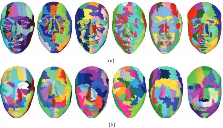
Step 1. Clustering. When considering that each vertex normal is computed using the data in a local neighborhood that is independent of the face pose, we perform clustering that is based on the directions of the vertex normals. We usek-means clustering [39] to obtain a cluster setC={c1, c2, c3,· · · , ck}. Figs. 2.(a), 3.(a) and 4.(a) show our results on different 3D face databases. The k value of the k-means clustering is set to 15 empirically.

From the figures, we observe that the vertices on a given side of the nose are assigned to the same cluster, as we would expect. This result is crucial because the nose is detected by finding the specific clusters on its two sides. However, note that some vertices from other regions of the face (e.g., a cheek) are assigned to the same cluster as the nose vertices. In addition, there are many small clusters that have only a few vertices. These problems make it difficult to detect the nose. For better detection, a graph-based partitioning algorithm is used to edit the clusters that are obtained using thek-means algorithm.

Algorithm 1 Graph-based Partitioning Algorithm

Input:Face meshF=< V, E >,

Cluster setC={c1, c2, c3,· · ·, ck},

Edge weight listW ={w1, w2, w3,· · ·, wm},

Minimum patch size thresholdλ.

Output:Patch setP ={p1, p2, p3,· · ·, pn}

1. begin

2. P={}

3. fori= 1→kdo begin

4. Divideciinto patches based on the connectivity and obtain

5. the patch setPiP =Pi∪P

6. end for

7. fort= 1→mdo begin

8. Get the edgeeij= (vi, vj)according to the weightwt

9. Find patchpiand patchpj, wherevi∈piandvj∈pj

10. ifpi̸=pjandmin(size(pi),size(pj))< λ

11. Mergepiwithpjand updateP

12. else

13. Continue

14. end if

15. end for

16. returnP={p1, p2, p3,· · ·, pn}

17. end

Step 2. Graph-based Partitioning. The graph-based par-titioning algorithm merges small clusters. Let F = (V, E)

denote a 3D face mesh that has a set of vertices V and a set of undirected edges E. Each edge eij ∈ E is a pair of adjacent vertices (vi, vj) that has a corresponding weight

w(eij), wherevi, vj∈V. The edge weight is a measure of the distance between two adjacent vertices. The weight of an edge that connects two adjacent vertices from the same cluster is zero. For an edgeeij that connects two adjacent vertices from different clusters, the weight is calculated as follows:

w(eij) =e−cosθ (2)

whereθis the angle between the normal vectorsviandvj. A larger angle yields a larger value for the weight. Considering we have

cosθ= ni·nj

|ni||nj|

(3)

where ni and nj are unit normal vectors of vi and vj, and

(5)

(a)

[image:5.612.128.485.54.259.2]

(b)

Fig. 2. Results of the face partitioning on the BU-3DFE database. (a) Results ofk-means clustering, in which every color represents a cluster. (b) Results of the Graph-based Partitioning Algorithm, in which every color represents a patch.

(a)

[image:5.612.117.498.301.507.2]

(b)

Fig. 3. Results of the face partitioning on the GavabDB database. (a) Results of thek-means clustering, in which every color represents a cluster. (b) Results of the Graph-based Partitioning Algorithm, in which every color represents a patch.

w(eij) =e−

|ni||nj|

ni·nj ₌_e−ni·nj ₍₄₎

The edges that have zero weight are deleted and the remaining weights are sorted ascendingly into a list W =

{w1, w2, w3,· · ·, wm} according to the edge weight values. As mentioned above, vertices from different parts of the 3D face can be included in the same cluster, which will cause difficulties in nose detection. To solve this problem, we separate the vertices within each cluster by accounting for the spatial connectivity. Every cluster is divided into a number of small patches, such that the vertices in each patch form a connected sub-graph of the original triangulation. Let the set of patches be P = {p1, p2, p3,· · ·, pn}. We define the size of a patch as the number of vertices in the patch. Patches that are too small are removed by iterative merging.

A minimum patch size threshold λ is used to filter out the small patches. During the iterative process, every small patch that has a size below λ is merged with the nearest adjacent patch. Additionally the nearest adjacent patch is identified as the patch that is connected to the small patch by the edge that has the smallest weight. The merging process terminates when the size of each patch is larger thanλ. Empirically, the vertices of the nose make up approximately 6% of the total vertices of the 3D face; hence, in practice,λis set to0.03N

in our approach, where N is the total number of vertices in the 3D face. The final result is that the face is covered by a few large patches and each side of the nose corresponds to an individual patch. The graph-based partitioning algorithm is described in Algorithm 1.

(6)

(a)

[image:6.612.119.496.55.276.2]

(b)

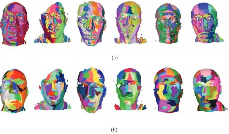
Fig. 4. Results of the face partitioning on the FRGC 2.0 database. (a) Results ofk-means clustering, in which every color represents a cluster. (b) Results of the Graph-based Partitioning Algorithm, in which every color represents a patch.

Graph-based Partitioning Algorithm. In each figure, each color represents a patch, and as observed, the 3D faces are covered by a relatively small number of large patches, and the nose region is partitioned into two patches, one on each side of the nose. Using the partitioning result, we can easily detect the nose by selecting the two patches and combining them.

3) Feature Descriptor: To select the nose patches, we must find a descriptor that can differentiate the nose patches from other patches. Because of the distinctive shape of the nose, spin images [40] that are calculated at each inner vertex are utilized to describe a patch.

A spin image is a local shape descriptor that is initially introduced by Johnson and is used for surface matching. It is very similar to a space histogram and describes the relative distance between an oriented point and other points.

We use the mean of the spin images (MSI) to represent a patch. The MSI in a patch is defined as follows:

M SIPr = 1

|Pr| ∑

pi∈Pr

Spi (5)

where|Pr|is the number of vertices in the patchPr, andSpi

is the spin image at vertexpi. Because MSI accounts for all of the vertices in the patch, it offers an advantage for overcoming problems that are caused by noise, local deformation and resolution. In addition, MSI is robust to the pose variations because the spin images are object-centered representations. Fig. 5 shows examples of the MSIs of different patches. Fig. 5 (a) and (b) are spin images for the two sizes of the nose; (c) is for the left cheek; and (d) is for the right jaw.

4) Feature Detector: To detect the two nose patches, we must determine whether a patch is a part of the nose. This determination is a binary classification problem, and many methods have been proposed to address this issue. In our approach, we use a detector that is based on the popular SVM classifier [41]. The detector is generated by supervised

(a) (b)

(c) (d)

Fig. 5. MSIof different patches.

training that utilizes the MSIs for different patches. We label the patches manually for training the SVM classifier.

Our detector is applicable to a wide range of different 3D faces because the MSIs of the nose patches are similar for all of the 3D faces. Based on the output of the detector, only two patches are selected. The two selected patches are merged to obtain the nose region. Experimental results for the nose detection are given in Section IV.

B. Coarse Alignment

Once the location of the nose in the point cloud is known, alignment of the input face is possible. However, because our nose detection algorithm focuses on the whole nose region and the number of selected vertices for each input face is different, the 3D vertices in the nose region are unordered. It is difficult to obtain an accurate alignment using these vertices. In other words, only a coarse alignment is achieved for a 3D face alignment that is based on the nose.

[image:6.612.329.545.322.451.2]

(7)

vr=t+R(α1, α2, α3)·s·vt (6) wherevtandvrdenote the corresponding vertices on the test face and reference face; t denotes the translation vector;α1,

α2, α3 denote the three rotation parameters; R denotes the

total rotation matrix; and sdenotes the scale factor.

The rotation matrix is an orthogonal matrix that is the product of three individual rotation matrices:

R(α1, α2, α3) =R1(α1)·R2(α2)·R3(α3)

where α1, α2 and α3 are the rotation angles that are along

the x,y andz axes, respectively. As described in [43], three control vectors are needed to obtain the rotation matrix in (6). In our approach, the rotation matrix is computed based on the detected nose. Given the two patches on either side of the nose, we first extract the average normals for each patch as follows

nPr = 1

|Pr| ∑

vi∈Pr

ni (7)

where ni is a unit normal vector at the vertex vi and|Pr| is the number of vertices in patchPr.

Afterwards, we can obtain the third vector from the cross product of the two normal vectors. Given three mutually orthogonal vectors for the test face and reference face, the rotation matrix can be obtained.

The translation vector t can be obtained by computing the distance between the center of the bounding boxes for each nose. The scale factor s is estimated using the ratio of the sizes of the two bounding boxes.

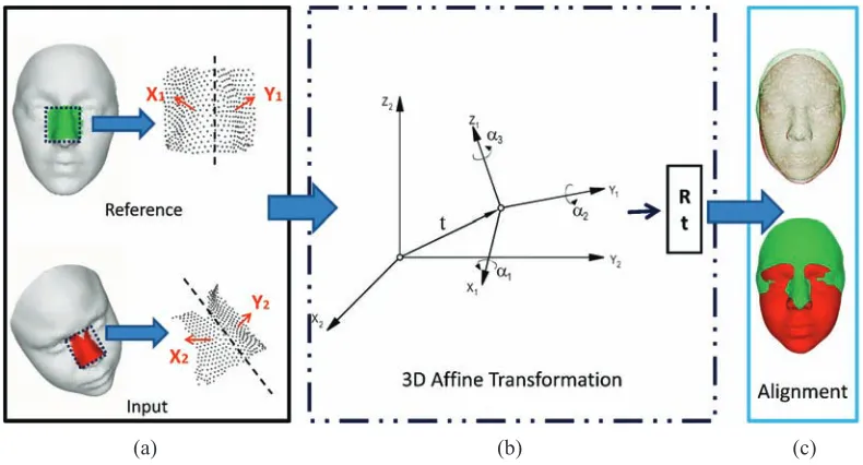
Fig. 6 describes the work flow of our 3D face coarse alignment process.

C. Fine Alignment

Because only the nose vertices are involved in the coarse alignment, the normal vectors that are used to define the 3D affine coordinate transformation cannot exactly represent the orientation of the face. The coarse alignment is not sufficiently accurate to build the correspondences between the features of the test face and reference face. In our approach, an Iterative Closest Point (ICP) algorithm [2] is used to further refine the alignment. Because the expression of the test face is unknown, it is desirable to have a reference 3D face set F that consists of different expressions of a subject to perform the fine alignment.

The Iterative Closest Point (ICP) algorithm [2] has been proven to be valid for matching different 3D faces [45]. In our approach, the ICP algorithm is used to improve the alignment. The ICP algorithm is an iterative procedure for aligning two free-form shapes by minimizing the mean square error between the points in the test face ft and the closest points in the reference facef_rm∈ F. The algorithm terminates when the iteration exceeds a preset threshold. In our approach, the preset iteration number is set to 30 empirically. The algorithm outputs the affine transformation, including the rotation matrix

R, translation vectort and scale parameter S. Only the face

fm

r that has the smallest error in F is chosen as the final reference face. After employing the ICP algorithm, the affine transformation parameters are applied to ft to align it as closely as possible with the reference facefm

r .

In the fine alignment, given a 3D face ft that has an unknown expression, the ICP algorithm helps us to find the most suitable facef_rmin the reference 3D face setF and align

ft tofrmin an iterative way.

Please note thatFis only a fraction of the training database, which is composed of 25 expressive faces from one subject in the training database. In the training database, all of the 3D faces are pre-aligned well for the purpose of sharing the same number of vertices and the same topology.

III. STAGETWO: LANDMARKLOCALIZATION BASED ON

LOCALCOORDINATECODING

The key aim of LCC-based landmark localization is to obtain the 3D coordinate of the landmarks of the input 3D face. In our approach, we first perform re-sampling to establish the dense vertex-wise correspondences between the input face and training database. Then, based on the 3D faces in the training database and their corresponding landmarks, we learn a coupled dictionary to model the relationship between the point cloud and the landmarks based on Local Coordinate Coding (LCC) [27]. Afterward, given the test 3D face, we can synthesize the 3D coordinate of the landmarks based on the learned coupled dictionary. Finally, the landmarks on the given test 3D face can be located under the guidance of the synthesized landmark coordinates.

A. Face Re-sampling

After alignment, the input 3D face is re-sampled by using the reference 3D face. The re-sampling involves the projection of each face onto a cylinder [30]. Fig. 7 illustrates the pipeline of the two-step re-sampling algorithm.

1) Cylindrical projection: After face alignment, the input face ft and reference face frm are projected onto a cylinder. For a vertex p= [xo, yo, zo]T, its cylindrical coordinates after projection are (uo, vo), where uo =

arccos(xo/r), andr= √

x2

o+zo2,v0=y0.

2) Mesh image and re-sampling: To build the correspon-dence between the input faceft and its reference face

fm

r , each vertex inftmust be matched to a correspond-ing vertex in the reference face. To achieve this dense vertex-wise correspondence, we perform interpolation of the cylindrically projected ft to obtain a high-resolution mesh image. Based on the cylindrical coor-dinates, the reference face can perform re-sampling on the mesh image. Finally, the re-sampled test 3D face is obtained, which has dense vertex-wise correspondence with the training face.

(8)

[image:8.612.109.504.53.266.2]

(a) (b) (c)

Fig. 6. Process of coarse alignment. (a) The reference face and input face. (b) 3D affine transformation. (c) Results of the coarse alignment.

Reference Mesh Image

Mesh Image Input Faces

Correspondence

Fig. 7. Pipeline of 3D face re-sampling.

B. Coupled Dictionary Learning for Local Coordinate Coding

It is known that the landmarks occupy the important lo-cations in the 3D face in such a way that they cover and describe the shape of the 3D face. In our coupled dictionary learning for local coordinate coding (LCC), we assume the 3D faces and their corresponding landmark sets from manifolds have similar local geometries in two different spaces [28], [29], [32]. Hence, we concatenate each training 3D face and its corresponding landmark set together as a sample. Given a sample x = {xf, xl}, we define xf as the training 3D face, which contains N vertices, and xl as its corresponding landmark set, which containsLvertices. Each vertex is defined with the 3D coordinatevi= (lxi, l

y i, l

z

i). Thus, each input face is converted into a 3N×1 vector, and the landmark set is a

3L×1vector forLlandmarks. The LCC finds the best coding

α(x) ∈RM for x, which minimizes the reconstruction error and the violation of the locality constraint. This concept can be formulated as follows:

min

D_∈C,α

1

2||x−Dα||

2₊_µ∑

j

|αj|∥dj−x∥2 (8)

whereC={D|∥di∥ ≤1, i= 1, . . . , M}is the convex feasible set of D. D = [d1, d2,· · · , dM] ∈ R3(N+L)×M is a set of

bases or a dictionary. Here,di=df(i), dl(i), anddf(i),dl(i) are 3D face and landmark sets, respectively. It is important to constrain the columns ofD because we can fix Dα and the scale of D to make ∑_j|αj_|∥_d

j−x∥2 arbitrarily small. The first term of the objective function measures the reconstruction error, and the second term preserves the locality of the coding. Given a set of samples{x1, x2,· · · , xn} ∈R3(N+L), the bases or dictionary D= [d1· · ·dM]∈Rh×M can be learned by linearly approximating these samples as (8). For dictionary learning, we can minimize the summed objective function of all data samples overDandαsimultaneously [33], [34], i.e.,

min

D∈C,αi

∑

i (

1

2||xi−Dαi||

2₊_µ∑

j

|αj_i|∥dj−xi∥2 )

(9)

wherexi is thei-th sample andαiis its corresponding coding coefficient.

However, the above objective function is not jointly convex overDandα, which makes it difficult to solve. Nevertheless, it is convex over D with fixed α and vice versa. Therefore, we can optimize overD while keeping the value ofαi fixed, and then, we can optimize over αi while keeping the value ofD fixed. This alternating set of optimizations is performed until convergence.

For a fixed dictionaryD and a sample x, optimizing over

αcan be transformed into optimizing the following equation overβ:

min

β

1

2||x−DΛ

−1_β_||2₊_µ_∥_β_∥

1 (10)

where Λ is a diagonal matrix whose diagonal elements are

Λjj =||dj−x||2 andβ = Λα, and||β||1=

∑

j|βj| denotes the l1-norm. In addition, we assume that dj ̸=x; thus, Λ−1 exists. After solvingβ, we can obtain α= Λ−1_β_{. Here,} _α_is

[image:8.612.48.300.304.426.2]

(9)

3D Faces

Facial Masks Input

Code

Output Combination

Dictionary

[image:9.612.130.484.53.274.2]

Dictionary

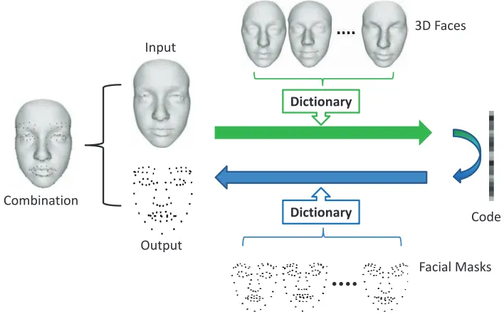
Fig. 8. Procedure for landmark localization.

For a fixedα, optimizing overD is a constrained quadratic programming problem. By expanding the squares in Eq. (9) and dropping the terms that do not haveD, we can obtain

D=arg min

D_∈C ∑

i (

1

2||xi−Dαi||

2₊_µ∑

j

|αj_i|∥dj−xi∥2 )

=arg min

D_∈C

1 2tr

[

DTD( ∑

i

αiαiT + 2µΣi )]

−tr [

DT· ( ∑

i

xiαiT + 2µxiα¯Ti )]

(11)

where α¯i is the component-wise absolute value of αi, i.e.,

¯

αj_i = |αj_i|, and Σi is a diagonal matrix that is constructed from αi.

Define two matrices, A = ∑_iαiαiT + 2µΣi and B = ∑

ixiαiT + 2µxiα¯Ti . Then, the optimal D can be found by performing a block-coordinate descent. In iteration k of the dictionary update, we update the j-th column dk_j when the other columns are fixed. Denote aj and b−j as the j-th columns of the matricesAandB,ajj as the(j, j)-th element of A, and the dictionaryDk at iterationk. The updating rule is as follows

dk_j+1= Π

( dk_j − 1

ajj (

Dkaj−bj ))

(12)

whereΠ(·)is the projection operator onto the feasible set of

D.

The detail of the coupled dictionary learning algorithm is given in Algorithm 2.

C. Landmark Localization

In contrast to the previous feature detection-based method and the statistical PDM-based method, in our approach, we synthesize the landmarks first instead of detecting or fitting

Algorithm 2 Coupled Dictionary Learning

Input:Training database{x1, x2,· · ·, xn},

Initial dictionaryD0,µ. Output:Learned dictionaryDn Initialize:A0←0,B0←0

1. fort←1tondo

2. Draw a samplext from the training database.

3. Local coordinate coding: compute using Eq. (10)

αt= arg minα1₂∥xt−Dt−1α∥2+µ∑j|αj|∥(Dt−1)j−xt∥2

4. UpdateAt←At−1+αtαTt + 2µΣt.

5. UpdateBt←Bt−1+xtαTt + 2µxtα¯Tt.

7. Update dictionary using Eq. (12) dtj= Π

(

dt_j−1−_a1 jj

(

Dt−1aj−bj)).

8. end for

9. returnDn

them through some local feature descriptor or statistical point distribution model. This concept enables us to perform the landmark localization robustly over the whole face and to adapt to changes in the extent to which the 3D data cover the face.

As Fig. 8 shows, some sample faces and their corresponding landmarks are selected as the training data to learn the two dictionaries for the LCC.

Given that the coupled dictionary is learned, let xf be an input 3D face, letDf be the 3D face dictionary, and letαbe the coefficients of Df. The approximation toxf can then be formulated as follows:

x′_f =∑Dfα (13)

(10)

minc ∑

x∥xf−Dfα∥2

s.t. 1T_α_{= 1} ₍₁₄₎

As discussed in Section III-B, we assume that the 3D faces and their corresponding landmark sets form manifolds that have similar local geometries in two different spaces [32]. Hence, we can approximate the corresponding landmark set

xlby using the same coefficients forx

′

f. By replacing the 3D face dictionary Df with the landmark dictionaryDl, we can obtain the corresponding synthesized landmark set x′_l:

x′_l=∑Dlα (15)

Considering that x′_l is synthesized based on dictionaryDl, it is clear that x′_l is not exactly equal to the landmark setxl, even though it is very close to it. It is desirable to employ vertices that are in the 3D face instead of synthesized vertices to be the landmarks. Thus, in our approach, we further find the vertices that are closest to the synthesized landmarks to be our localization result. Given x′_l = {v_i′}1≤i≤L and xl =

{vi}1≤i≤L,

vi= min vj

∥v_i′−vj∥2 (16)

wherevj ∈xf

Finally through the above steps, each input 3D face is marked with the corresponding landmarks.

IV. EXPERIMENTALRESULTS

A. Database

In this section, we test our method on the BU-3DFE database [35], GavabDB database [36] and FRGC 2.0 database [37]. The experimental results are demonstrated in the follow-ing subsections.

The BU-3DFE database contains 100 subjects (56%female,

44% male), who range in age from 18 to 70 years and who have a variety of ethnic/racial ancestries. There are 25 instant 3D expression models for each subject, which results in a total of 2,500 3D facial expression models. In addition, the BU-3DFE database provides 83 landmarks for each 3D face, which help us to train and test our proposed landmark localization method.

The GavabDB database contains 549 3D images of facial surfaces. The meshes in the database correspond to 61 different individuals with different poses and facial expressions.

The FRGC 2.0 database is sponsored by several government agencies and contains hundreds of frontal 2D face images and 3D face meshes. Different poses and expressions are observed in the 3D faces.

Note that because the proposed method is based on nose detection, we chose only the 3D faces that have noses in our experiments.

B. Nose Detection

Before conducting the experiments, 50 faces from various ancestries and with various expressions are selected for train-ing an SVM model. Because the MSI of the nose patches differs greatly from those of other patches, as Fig. 5 shows, a simple linear kernel is used in the SVM classifier. After detection, the detected noses are shown in red on the frontal faces for better display.

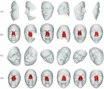
For the nose detection on the BU-3DFE database, the testing faces can be divided into two sets. Set 1 consists of faces that have only yaw rotations, slight expression variations and missing data. Set 2 consists of faces that have combinations of yaw rotation, pitch rotation, roll rotation, and extreme expression variations. Because the 3D faces in the BU-3DFE database are frontal, we rotate these models for evaluation.

Some representative experimental results that are obtained from Set 1 and Set 2 are shown in Fig. 9. Figs. 9 (a) and (b) illustrate the nose detection results for Set 1. As the figure shows, our approach correctly detects the noses of 3D faces that have different yaw rotations and expressions, even when there is a hole that is caused by missing data. Figs. 9 (c) and (d) illustrate the nose detection results for Set 2. Faces from Set 2 have combinations of yaw rotation, pitch rotation and roll rotation along with extreme expression variations. As the figure shows, our approach still correctly detects the noses of the 3D faces.

To validate the proposed nose detection method, we exper-iment further with the GavabDB and FRGC 2.0 databases. These two databases consist of many originally non-frontal faces. Collars, necks and missing data are challenges for our proposed nose detection method. Some representative experimental results are shown in Figs. 10 and 11.

C. Face Alignment

Nairet al.[4] also presented an ICP-based 3D face align-ment approach, in which the curvature information is utilized to find the facial features to make a coarse alignment before performing the ICP-based fine alignment. To evaluate the performance of our approach, we make a comparison between the Nairet al. approach and our approach.

The alignment is successful when the average pixel-wise error between the test face and reference face is less than 2 mm. The alignment rate is the ratio between the number of successfully aligned faces and the total number of tested faces. All of the methods have been programmed using Matlab 7.11 on a PC with an Intel(R) Core(TM)2 Duo CPU E5800 3.16 GHz and 4 GB RAM. Here, 1500 3D faces from different databases are used for testing.

In the evaluation, 1500 faces are randomly selected from the three databases for testing. Both neutral and expressive 3D faces are included. Each 3D face is rotated around thex -axis,y-axis andz-axis. The angle of rotation around each axis is generated randomly and ranges from−πtoπ. We divide the testing faces into three groups according to their expressions: neutral, mild and extreme.

(11)

(a)

(b)

(c)

[image:11.612.128.487.55.364.2]

(d)

Fig. 9. (a) Examples of 3D faces in Set 1. (b) The nose detection results of Set 1. (c) Examples of 3D faces in Set 2. (d) The nose detection results of Set 2. Note that the nose detection results are shown by rotating the input faces into frontal views.

(a)

[image:11.612.125.489.406.546.2]

(b)

Fig. 10. (a) Examples of input 3D faces. (b) The nose detection results of the GavabDB database.

(a)

(b)

[image:11.612.127.492.578.724.2]

(12)

TABLE I

PERFORMANCE OF NOSE DETECTION BASED3DFACE ALIGNMENT

Expression Neutral Mild Extreme

Samples 512 603 385

Error (mm) mean std. <2 mm mean std. <2 mm mean std. <2 mm Nairet al.[4] 2.07 1.74 77.4% 3.13 2.54 67.3% 5.15 3.75 50.9%

Ours 1.45 1.27 94.5% 1.97 1.51 93.7% 2.45 1.93 80.8%

TABLE II

ACCURACY COMPARISON ON THE ROTATED NEUTRAL3DFACES(OCFOR OUTER CONTOUR, OULFOR OUTER UPPER LIP, OLLFOR OUTER LOWER LIP,

ILLFOR INNER LOWER LIP, IULFOR INNER UPPER LIP, LEFOR LEFT EYE, REFOR RIGHT EYE, NEFOR NOSE, LEBFOR LEFT EYE-BROW, REBFOR RIGHT EYE-BROW.)

Method RF-AAM [16] PDM [4] SS-PDM [10] Ours

Error <5 mm mean std. <5 mm mean std. <5 mm mean std. <5 mm mean std. OC 84.5% 3.38 3.35 33.0% 8.95 7.85 72.1% 4.21 2.36 91.2% 2.91 2.01 OUL 83.4% 3.50 2.51 35.0% 8.47 7.12 63.5% 5.12 3.32 88.7% 3.05 2.23 OLL 85.8% 3.22 2.31 26.1% 11.73 10.11 62.8% 5.21 3.23 85.3% 3.31 2.21 ILL 87.6% 3.12 2.15 25.6% 12.26 11.12 62.0% 5.32 3.31 89.2% 2.89 2.16 IUL 87.1% 3.14 2.13 29.4% 10.57 10.14 66.0% 4.75 3.01 88.9% 2.91 2.15 LE 86.6% 3.17 2.57 37.3% 7.75 6.75 74.5% 4.05 2.24 93.1% 2.59 2.31 RE 87.4% 3.13 2.55 37.8% 7.28 6.73 73.3% 4.12 2.57 93.0% 2.61 2.33 NE 78.8% 3.77 2.79 79.7% 3.75 2.23 88.4% 3.09 2.21 93.4% 2.55 2.22 LEB 77.6% 3.87 2.80 26.6% 11.63 10.73 66.5% 4.73 2.41 88.3% 2.99 2.84 REB 77.7% 3.86 2.83 26.6% 11.62 22.23 67.4% 4.53 2.34 89.2% 3.03 2.82

TABLE III

ACCURACY COMPARISON ON THE ROTATED MILD EXPRESSIVE3DFACES.

TABLE IV

ACCURACY COMPARISON ON THE ROTATED EXTREME EXPRESSIVE3DFACES.

the corresponding vertices in the test face and reference face. Table I shows that our method outperforms Nairet al.method in all of the expression groups. Nair et al. method uses three thresholds to identify the salient high-curvature regions, concave regions and convex regions, which are not robust if there are large deformations in the 3D faces. In contrast, our approach is more robust to the variations in the expressions because the 3D shape of the nose is stable. Additionally, with regard to the run time, Nairet al.method takes 44.178 seconds to process one 3D face, while our method takes 9.71 seconds.

D. Landmark Localization

Comprehensive and quantitative evaluations have been performed in our experiments. Comparisons between

RF-AAM [16], Nair et al. work (PDM for short) [4], Perakis

(13)

TABLE V

ACCURACY COMPARISON ON THEBU-3DFEDATABASE FACES. EACH FACE CONTAINS APPROXIMATELY35KVERTICES.

TABLE VI

ACCURACY COMPARISON ON THE SUBSAMPLEDBU-3DFEDATABASE FACES. EACH FACE CONTAINS APPROXIMATELY8.7KVERTICES.

TABLE VII

ACCURACY COMPARISON OF THE INTERPOLATEDBU-3DFEDATABASE FACES. EACH FACE CONTAINS APPROXIMATELY140KVERTICES.

We use the BU-3DFE database to make the quantitative evaluation because it contains 100 subjects while posing six different expressions that have varying levels of intensity. Each 3D face contains approximately 35K vertices. More impor-tantly, each 3D face in the BU-3DFE database is annotated with the location of 83 landmarks, which can be used as the ground truth for the quantitative evaluation. A total of 1250 3D faces and their corresponding landmarks from 50 subjects in the BU-3DFE database are used as training data and the others for testing. For our LCC-based landmark localization, all of the training faces are preprocessed to have vertex-wise correspondence. And the average interpupillary distance (IPD) of the test faces is 68.9 mm. For the other existing methods, the training settings are the same as those in [16], [4] and [10]. In addition, we train a random forest [15] for the initialization of RF-AAM, as discussed in [16]. Apart from RF-AAM, the other landmarking methods, Nair et al. and Perakiset al. are trained according to [4] and [10], respectively.

To compare the tolerance to rotations and expressions, each 3D face of the testing data is rotated around the x-axis, y -axis and z-axis. The angle of rotation around each axis is generated randomly and ranges from −π to π. Additionally,

the testing data are divided into three groups in terms of their expression intensity: neutral, mild and extreme. The performance of RF-AMM, PDM, SS-PDM and our approach are given in Tables II, III and IV. The experimental results show that our approach outperforms the state of these art methods by providing more stable and accurate locations when there are different poses for the 3D face.

(14)

(a)

(b)

[image:14.612.111.501.59.341.2]

(c)

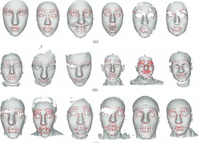
Fig. 12. Examples of our landmark localizing results on the (a) BU-3DFE, (b) GavabDB and (c) FRGC 2.0. databases

in pose, expression, resolution and face incompleteness. PDM and SS-PDM produce similar results on high-resolution data but are worse on low-resolution data. RF-AAM is sensitive to the variations in the resolution because both the template patch for the AAM training and the patch for the random forest-based posed estimation are fixed in size.

Examples of our landmark localizing results on the BU-3DFE database are given in Fig. 12(a). We also perform our landmark localization on the Gavab and FRGC 2.0 databases. The examples of the results are shown in Figs. 12(b) and (c). Some of the examples show that our approach can produce the landmarks robustly even in cases in which the 3D faces are not completely covered by the data.

V. CONCLUSIONS ANDFUTUREWORK

In this paper, we present a local coordinate coding-based approach to automatically locate the landmarks of a 3D face robustly and accurately. The proposed approach consists of two stages: nose detection-based 3D face alignment and LCC-based landmark localization. In the first stage, nose detection is accomplished by partitioning the 3D face into several patches and then selecting the nose patches using an SVM classifier. Once the nose is detected, a coarse alignment is obtained between the test face and reference face. This alignment is followed by an ICP-based fine alignment. In the second stage, we re-sample on a given 3D face to build a vertex-wise correspondence with the reference face and to obtain a training dictionary of the LCC-based landmark localization. Then, an LCC-based coupled dictionary learning algorithm for landmark localization is presented. Finally, the landmark

coordinates are obtained by finding the vertices that are closest to the synthesized landmarks based on the LCC.

The experimental results show that our method achieves high accurate landmark localization which is robust to vari-ations in the pose, expression, resolution and face incomplete-ness. In the future, we will expand our work to the area of 3D face recognition and facial expression synthesis based on alignments.

REFERENCES

[1] X. Lu, and A.K. Jain, “Automatic feature extraction for multiview 3D face recognition,”Proc. 7th Conf. Automatic Face and Gesture Recognition, 2006, pp. 585-590.

[2] P.J. Besl, and N.D. McKay, “A method for registration of 3-D shapes,” IEEE Trans. Pattern Anal. Mach. Intell., volume 14, 1992, pp. 239-256. [3] P. Perakis, T. Theoharis, G. Passalis, and I.A. Kakadiaris, “Automatic 3D facial region retrieval from multi-pose facial datasets,”Proc. Eurographics Workshop on 3D Object Retrieval, 2009, pp. 37-44.

[4] P. Nair, and A. Cavallaro, “3-D Face detection, landmark localization, and registration using a point distribution model,”IEEE Trans. Multimedia, volume 1, 2009, pp. 611-623.

[5] D. Colbry, G. Stockman, and A. Jain, “Detection of anchor points for 3D face verification,” IEEE Workshop on Advanced 3D Imaging for Safety and Security, 2005, pp. 118.

[6] T.H. Lin, W.P. Shih, W.C. Chen, and W.Y. Ho, “3D face authentication by mutual coupled 3D and 2D feature extraction,”Proc. 44th ACM Southeast Conference, 2006, pp. 423-427.

[7] M.P. Segundo, C. Queirolo, O.R.P. Bellon, and L. Silva, “Automatic 3D facial segmentation and landmark detection,”Proc. 14th Int. Conf. Image Analysis and Processing, 2007, pp. 431-436.

[8] C. Dorai, and A.K. Jain, “COSMOS - A representation scheme for 3D free-form objects,”IEEE Trans. Pattern Anal. Mach. Intell., volume 19, 1997, pp. 1115-1130.

(15)

[10] P. Perakis, G. Passalis, T. Theoharis, and I. A. Kakadiaris, “3D Facial Landmark Detection under Large Yaw and Expression Variations,”IEEE Trans. Pattern Anaysis and Machine Intelligence, 2012.

[11] H. Dibeklio˘glu, A.A. Salah, and L. Akarun, “3D Facial landmarking under expression, pose, and occlusion variations,”Proc. Int. Conf. Bio-metrics: Theory, Applications and Systems, 2008, pp. 1-6.

[12] M. Romero-Huertas, and N. Pears, “3D Facial Landmark Localisation by Matching Simple Descriptors,”Proc. Int. Conf. Biometrics: Theory, Applications and Systems, 2008, pp. 1-6.

[13] T.F. Cootes, C.J. Taylor, D.H. Cooper, and J. Graham, “Active shape models-their training and application,”Computer Vision and Image Un-derstanding, volume 61, No. 1, 1995, pp. 38-59.

[14] C. Creusot, N. Pears, J. Austin, “A machine-learning approach to keypoint detection and landmarking on 3D meshes,”International Jounal of Computer Vision, 102:147-179, 2013.

[15] G. Fanelli, M. Dantone, J. Gall, A. Fossati, and L. Van Gool, “Random forests for real time time 3D face analysis,” International Journal of Computer Vision, 101: 437–458, 2013.

[16] G. Fanelli, M. Dantone, and L. Van Gool, “Real time 3D face alignment with random forests-based active appearance models,”IEEE Conference on Automatic Face and Gesture Recognition, pp. 1-8, 2013.

[17] G. J. Edwards, C. J. Taylor, and T. F. Cootes. “Interpreting face images using active appearance models,”Proc. Int. Conf. Automatic Face and Gesture Recognition, June 1998, pp. 300-305.

[18] T. Cootes, G. Edwards, and C. Taylor. “Active appearance models,”Proc. European Conf. Computer Vision, volume 2, 1998, pp. 484-498. [19] T. Cootes, G. Edwards, and C. Taylor. “A comparative evaluation

of active appearance models algorithms,”Proc. British Machine Vision Conference, 1998, pp. 680-689.

[20] T. F. Cootes. “Statistical models of appearance for computer vision,” Online technical report available from http://www.isbe.man.ac.uk/ bim/refs.html, Sept. 2001.

[21] T. F. Cootes, G. J. Edwards, and C. J. Taylor. “Active appearance models,”IEEE Trans. Pattern Anal. Mach. Intell., volume 23, 2001, pp. 681-685.

[22] T. Cootes and P. Kittipanya-ngam. “Comparing variations on the active appearance model algorithm,” In Proceedings of the British Machine Vision Conference, volume 2, 2002, pp. 837-846.

[23] A. Batur and M. Hayes, “Adaptive active appearance models,” IEEE Transactions on Image Processing., vol. 14, no. 11, 2005, pp. 1707-1721. [24] J. Zhu, S.C.H. Hoi, E. Yau, and M.R. Lyu, “Automatic 3D face modeling using 2D active appearance models,” Proceedings of the 13th Pacific Conference Computer Graphics and Applications, 2005, pp. 133-135. [25] K.S. Cho, Y.G. Kim, and G.S. Shin, “Fast 3D face synthesis using

AAM, Advanced Intelligent Computing Theories and Applications,”With Aspects of Contemporary Intelligent Computing Techniques, 2007, pp. 1119-1125.

[26] C.W. Chen, and C.C. Wang, “3D active appearance model for aligning faces in 2D images,”Proceedings of the IEEE/RSJ Int. Conf. Intelligent Robots and Systems, 2008, pp. 3133-3139.

[27] K. Yu, T. Zhang, and Y. Gong, “Nonlinear learning using local co-ordinate coding,”Advances in Neural Information Processing Systems, volume 22, 2009, pp. 2223-2231.

[28] L. Shao, R. Yan, X. Li and Y. Liu, “From heuristic optimization to dictionary learning: a review and comprehensive comparison of image denoising algorithms,”IEEE Transactions on Cybernetics, vol. 44, no. 7, pp. 1001-1013, 2014.

[29] L. Zhang, X. Zhen and L. Shao, “Learning object-to-class kernels for scene classification,”IEEE Transactions on Image Processing, vol. 23, no. 8, pp. 3241-3253, 2014.

[30] M. Song, Z. Dong, C. Theobalt, H. Wang, Z. Liu, and H.P. Seidel, “A generic framework for efficient 2-D and 3-D facial expression analogy,” IEEE Trans. on Multimedia, volume 9, no. 7, 2007, pp. 1384-1395. [31] M. Song, C. Chen, J. Bu, T. Sha, “Image-based facial sketch-to-photo

synthesis via online coupled dictionary learning,”Information Sciences, vol. 193, 2012, pp. 233-246.

[32] D. Tao, X. Li, X. Wu, S. J. Maybank, “Geometric mean for subspace selection,”IEEE Trans. Pattern Analysis and Machine Intelligence, 2009, pp. 260-274.

[33] R. Yan, L. Shao and Y. Liu, “Nonlocal hierachical dictionary learning using wavelets for image denoising,”IEEE Transactions on Image Pro-cessing, vol. 22, no. 12, pp. 4689-4698, 2013.

[34] F. Zhu and L. Shao, “Weakly-supervised cross-domain dictiornary learn-ing for visual recognition,”International Journal of Computer Vision, vol. 109, no. 1-2, pp. 42-59, 2014.

[35] L. Yin, X. Wei, Y. Sun, J. Wang, and M.J. Rosato, “A 3D facial expression database for facial behavior research,” Proc. 7th Int. Conf. Automatic Face and Gesture Recognition, 2006, pp. 211-216.

[36] A. B. Moreno and A. Sanchez, “GavabDB: A 3D face database,”Proc. Workshop Biometrics on the Internet COST275, 2004, pp. 77-82. [37] P.J. Phillips, P.J. Flynn, T. Scruggs, K.W. Bowyer, J. Chang, K. Hoffman,

J. Marques, J. Min, and W. Worek, “Overview of the face recognition grand challenge,”Proceedings of the IEEE conference on computer vision and pattern recognition, 2005, pp. 947-954.

[38] S. Jin, R.R. Lewis, and D. West, “A comparison of algorithms for vertex normal computation,”VISUAL COMPUT. volume 21, 2005, pp. 71-82. [39] J. MacQueen, “Some methods for classification and analysis of

multi-variate observations,”Proc. 5th Berkeley Symp. Mathematical Statistics and Probability, volume 1, 1967, pp. 281-297.

[40] A.E. Johnson, “Spin-images: A representation for 3-D surface match-ing,” Ph.D. thesis, Robotics Institute, Carnegie Mellon University, 1997. [41] C.J.C. Burges, “A tutorial on support vector machines for pattern recognition,”DATA MIN. KNOWL. DISC., volume 2, 1998, pp. 121-167. [42] B. Guo, S. Gunn, R. Damper, J. Nelson ,“Customizing kernel functions for SVM-based hyperspectral image classification,” IEEE Transactions on Image Processing., vol. 17, no. 4, 2008, pp. 622-629.

[43] C.O. Andrei, “3D affine coordinate transformations,” MSc in Geodesy, School of Architecture and the Built Environment, Royal Institute of Technology (KTH), Stockholm, Sweden, 2006.

[44] Y. Hu, M. Zhou, and Z. Wu, “A dense point-to-point alignment method for realistic 3D face morphing and animation,”International Journal of Computer Game Technology, 2009.

[45] T. Russ, C. Boehnen, T. Peters, “3D face recognition using 3D alignment for PCA,”IEEE Conference on Computer Vision and Pattern Recognition, pp. 1391–1398, 2006.

Mingli Song (M’06-SM’13)is an Associate Pro-fessor in Microsoft Visual Perception Laboratory, Zhejiang University. He received the PhD degree in Computer Science from Zhejiang University, China, in 2006. He was awarded Microsoft Research Fel-lowship in 2004. His research interests include face modeling and facial expression analysis.

Dacheng Tao(M’07-SM’12) is Professor of puter Science with the Centre for Quantum Com-putation & Intelligent Systems and the Faculty of Engineering & Information Technology in the U-niversity of Technology, Sydney. He mainly applies statistics and mathematics for data analysis problems in data mining, computer vision, machine learning, multimedia, and video surveillance. He has authored and co-authored 100+ scientific articles at top venues including IEEE T-PAMI, T-NNLS, T-IP, NIPS, ICM-L, AISTATS, ICDM, CVPR, ICCV, ECCV; ACM T-KDD, Multimedia and T-KDD, with the best theory/algorithm paper runner up award in IEEE ICDM’07 and the best student paper award in IEEE ICDM’13.

(16)

Chun Chenis a Professor in the College of Com-puter Science, Zhejiang University. His research interests include computer vision, computer graphics and embedded technology.