Optimization of Zero-Order Markov
Processes with Final Sequence of States
Alexandru Lazari
Moldova State University, MD-2009, Chisinau,Republic of Moldova
∗Corresponding Author: [email protected]
Copyright c⃝2013 Horizon Research Publishing All rights reserved.
Abstract
In this paper the zero-order Markov processes with final sequence of states X and unit transition time are analyzed. The evolution time T(p) of these systems is studied, where p represents the distribution of the states of the system. The problem of minimization the expectation E(T(p)) is considered. This problem is reduced to a geometric program, which is efficiently solved using convex optimization based on interior-point methods. The main idea of the proof is to show that the expressionE(T(p)) + 1 is a posynomial function in variables which represent the components of distribution of the states that participate in final sequence of states. For some particular cases the explicit solution is obtained.Keywords
Zero-Order Markov Process, Final Sequence of States, Evolution Time, Geometric Pro-gramming, Posynomial Function, Convex Optimization, Interior-Point Methods1
Introduction
The discrete Markov processes are often used as mathematical models that describe various applied ac-tual problems from many important domains: economy, technique, biology, industry, medicine and others. Based on these stochastic systems, the researchers obtain new numerical methods and algorithms for solving the com-plex problems of the society.
The Markov stochastic systems were studied in many scientific papers. The main results regarding these sys-tems were described in [7], [8] and [20]. Some applica-tions were presented in [9], [11], [16], [17] and [22].
The stochastic systems with final sequence of states generalize the discrete Markov processes. For these sys-tems the stopping condition is defined, i.e., the system stops when it passes through given final sequence of states. Unlike Markov processes, the evolution time of stochastic systems with final sequence of states is finite and depends on realization of stopping condition. For these systems the problem of determining the main pro-babilistic characteristics of evolution time of the system is interesting. This problem was studied in [14] and [15],
where polynomial algorithms based on the main proper-ties of homogeneous linear recurrences, generating func-tion and numerical derivafunc-tion of regular rafunc-tional frac-tions were obtained. The main generalizafrac-tions of these systems were presented in [12], [13] and [15].
In this paper the zero-order Markov processes with final sequence of states and unit transition time are studied. These systems represent a particular case of stochastic systems with final sequence of states. They are also called stochastic systems with final sequence of states and independent states or strong memoryless stochastic systems with final sequence of states, since at every discrete moment of time the state of the system does not depend on previous states.
For these stochastic processes the efficient method for minimizing the expectation of the evolution time is ela-borated. This method is based on geometric program-ming approach, that reduces the problem to the case of convex optimization using interior-point methods.
Geometric programming was introduced in 1967 by Duffin, Peterson, and Zener in [6]. Wilde and Beightler in 1967 and Zener in 1971 contributed with many re-sults (see [24] and [25]) referred of many extensions and sensitivity analysis. A short history of geometric pro-gramming was presented by Peterson in [19].
A geometric program represents a type of optimiza-tion problem described by objective and constraint func-tions that have a special form. This form is characterized by following rules: the objective function and left-hand side of inequality constraints need to be posynomials and left-hand side of equality constraints needs to be mono-mials. Also, in standard form, the geometric program is a minimization problem with right-hand side of all constraints equal to 1 and all inequality constraints con-taining the ”≤” operator. A good tutorial on geometric programming was presented in [3].
2
Statement of the problem
In this paper a discrete stochastic system L with the set of possible states V, where |V| = N ≤ ∞, is considered. The state of the system at every discrete moment of time t = 0,1,2, . . . is denoted byv(t) ∈ V. The transition time of the system from the state uto another statev at every moment of timetis equal to 1. On the set V a distribution function p : V → [0,1] is defined, where p(v) represents the probability with which the system L starts its evolution from the state v∈V. Also, the transition of the system from arbitrary stateu∈V to another statev∈V at every moment of timetis performed with probabilityp(v)∈[0,1].
The finishing evolution of the system is conditioned by passing consecutively through fixed sequence of states X = (x1, x2, . . . , xm) ∈ Vm. Let T be the stopping
time of the discrete stochastic system L. The value T represents the evolution time of the stochastic systemL. The systemLrepresents a zero-order Markov process with final sequence of states X and distribution of the statesp. For this system the moments of positive integer ordernof the evolution time are studied in [14] and [15]. In particular case the expectation of evolution time is obtained.
Next, we consider that the distributionpis not fixed. So, we have the zero-order Markov process L(p) with final sequence of statesX and distribution of the states p, for everypfrom the set
P ={y= (y1, y2, . . . , yN)∈[0,1]N |
N
∑
j=1
yj= 1}.
The problem is to determine the optimal distribution p∗∈ P, that minimizes the expectation of the evolution timeT(p) of the stochastic systemL(p), i.e.
T(p∗) = min p∈PT(p).
In the following chapters we will show how this problem can be solved using geometric programming.
3
Definitions and notations
3.1
Geometric programmingThe definition of geometric program requires the de-finition of monomials and posynomials.
Definition 1. In the context of geometric programming, a monomial is defined as a function f :Rs →Rof the
form f(x1, x2, . . . , xs) = cxα11 x
α2
2 . . . x
αs
s , where c > 0
andαi∈R,i= 1, s.
Definition 2. A posynomial is defined as a linear com-bination of monomials, i.e. represents a function of the
form f(x1, x2, . . . , xs) =
K
∑
k=1
ckxα1k
1 x
α2k
2 . . . xαssk, where ck>0,k= 1, K andαik∈R,i= 1, s,k= 1, K.
Posynomials are closed under addition, multiplication, and nonnegative scaling. Posynomials are not the same as polynomials, since:
• a polynomial’s exponents must be non-negative in-tegers, but a posynomial’s exponents can be arbi-trary real numbers;
• a polynomial’s coefficients can be arbitrary real numbers, but a posynomial’s coefficients must be positive real numbers.
Using these notions, we can define a geometric pro-gram in the following way.
Definition 3. A geometric program is an optimization problem of the form:
f0(x1, x2, . . . , xs)→min,
subject to
fi(x1, x2, . . . , xs)≤1, i= 1, r
hj(x1, x2, . . . , xs) = 1, j= 1, l
xk >0, k= 1, s ,
where fi(x1, x2, . . . , xs), i = 0, r, are posynomials and hj(x1, x2, . . . , xs),j= 1, l, are monomials.
In order to efficiently solve a geometric program we need to convert it to a convex optimization problem. Ef-ficient solution methods for general convex optimization problems were developed by Boyd and Vandenberghe in [4]. The conversion is based on a logarithmic change of variablesyk= lnxk,k= 1, sand a logarithmic transfor-mation of the objective and constraint functions. The obtained convex optimization problem has the form:
lnf0(ey1, ey2, . . . , eys)→min,
subject to
{
lnfi(ey1, ey2, . . . , eys)≤0, i= 1, r lnhj(ey1, ey2, . . . , eys) = 0, j= 1, l .
Unlike the original problem, the obtained problem looks more complicated, but it is convex and can be solved very efficiently using standard interior-point methods (see [3] and [4]). Also, the interior-point me-thods for solving geometric programs are very robust, require no starting point or other parameters and al-ways find the globally optimal solution of the problem.
3.2
Homogeneous linear recurrencesNext, we remind some definitions and notations from [12], [14] and [15] regarding homogeneous linear recurrences. We consider a subfield K of the fieldC.
Definition 4. The sequence a={an}∞n=0⊆C is called non-degenerated homogeneous linear m-recurrent sequence on the set K if there exists the vec-tor q= (qk)mk=0−1∈Km such that qm−1 ̸= 0 and
an= m∑−1
k=0
qkan−1−k, for all n≥m.
Definition 5. The vector q from previous defini-tion represents the generating vector and the vector
Im[a] = (an)mn=0−1 is called initial state of the sequencea.
• Rol[K][m] is the set of non-degenerated homoge-neous linearm-recurrent sequences on the setK;
• G[K][m](a) represents the set of generating vectors of lengthmof the sequencea∈Rol[K][m].
Definition 6. The functionG[a](z) = ∑∞
n=0
anzn is called
generating function of the sequence a = (an)∞n=0 ⊆ C
and the functionG[ta](z) = t∑−1
n=0
anzn is called partial
ge-nerating function of ordert of the sequencea.
Definition 7. Let a∈Rol[K][m]and q∈G[K][m](a). For the sequenceawe will consider the unitary characte-ristic polynomialHm[q](z) = 1−zG
[q]
m(z). For an arbitrary α ∈ K∗ the polynomial Hm,α(z) =[q] αHm[q](z) is called
characteristic polynomial of the sequencea.
Also, the following notation is introduced:
• H[K][m](a) is the set of characteristic polynomials of degreemof the sequencea∈Rol[K][m]. The next theorem presents the formula for the gene-rating function.
Theorem 1. If a ∈ Rol[K][m] and q ∈ G[K][m](a),
thenG[a](z) =
G[ma](z)− m∑−1
k=0
qkzk+1G[a]
m−1−k(z) Hm[q](z)
.
4
Preliminary results
4.1
Distribution of evolution timeThe zero-order Markov processes with final sequence of states were described in Section 2 and the evolution time T(p) of the system was defined. Let us consider the distributiona= (P(T(p) =n))∞n=0.
In [14] and [15], the properties of sequence a were studied. We obtained thata∈Rol[R][m] for p(x1)̸= 1
and p(xj) ̸= 0, j = 1, m. Also, we obtained formu-las for the initial stateIm[a] and the minimal generating vector q ∈ G[R][m](a). The established algorithm was described in the following way.
Algorithm 1.
Input: X = (xj)mj=1∈Vm,πj =p(xj), j= 1, m. Output: Im[a],q∈G[R][m](a).
1. The valueswk= k
∏
j=1
πj,k= 1, m, are determined.
2. The initial state Im[a]= (0,0, . . . ,0, wm)and the
va-luesu1,0= 1−π1 andv1,0=1 are calculated.
3. For eachs= 2, mthe following steps are executed: (a) The values
t(s) = min({t∈ {2,3, . . . , s+ 1} |
xt−1+j =xj, j = 1, s+ 1−t}),
are obtained.
(b) The parameters
vs,k= 0,k= 0, t(s)−3;vs,t(s)−2=
wt(s)−1
π1
;
vs,k=−wt(s)−1 π1
s−t∑(s)+1
j=k−t(s)+2
uj,k−t(s)+1,
k=t(s)−1, s−1, are calculated. (c) The quantities
us,k=π1(vs−1,k−vs,k),k= 0, s−2; us,s−1=−π1vs,s−1, are determined.
4. The components q0 = 1−π1vm,0, qk = −π1vm,k, k= 1, m−1, of generating vector q∈ G[R][m](a), are calculated.
In the case when exists j ∈ {1,2, . . . , m} such that p(xj) = 0, the evolution time is infinite. Also, the case p(xk) = 1,k= 1, m, is trivial. In this case the evolution time is equal to m−1, i.e., P(T(p) =m−1) = 1 and P(T(p) =n) = 0, for alln∈N\{m−1}.
4.2
Simplified version of Algorithm 1Next, we eliminate the parameters usk, s= 1, m, k= 0, s−1, from Algorithm 1. The following theorem holds.
Theorem 2. If one assumes the notations from Section 4.1, then the formula
vsk =
0, 0≤k≤t(s)−3
wt(s)−1
π1
, k=t(s)−2
−wt(s)−1
π1
(1−π1),
t(s−t(s) + 1) = 2 and k=t(s)−1
−wt(s)−1
π1
, t(s−t(s) + 1)≥3 and k=t(s)−1 wt(s)−1vs−t(s)+1,k−t(s)+1, t(s)≤k≤s−1
is true.
Proof. The particular case k ≤ t(s)−2 is trivial from Algorithm 1. Next, we consider the case k≥t(s). We have:
vsk=−wt(s)−1 π1
s−∑t(s)+1
j=k−t(s)+2
uj,k−t(s)+1
=−wt(s)−1 π1
(
uk−t(s)+2,k−t(s)+1
+
s−∑t(s)+1
j=k−t(s)+3
uj,k−t(s)+1
=−wt(s)−1 π1
(
−π1vk−t(s)+2,k−t(s)+1
+
s−∑t(s)+1
j=k−t(s)+3
π1(vj−1,k−t(s)+1−vj,k−t(s)+1)
=−wt(s)−1 π1
(
−π1vk−t(s)+2,k−t(s)+1
+π1(vk−t(s)+2,k−t(s)+1−vs−t(s)+1,k−t(s)+1)
)
In the case whenk=t(s)−1, we obtain
vsk=−wt(s)−1 π1
s−∑t(s)+1
j=1
uj0
=−wt(s)−1 π1
u1,0+
s−∑t(s)+1
j=2
uj0
=−wt(s)−1 π1
1−π1+
s−∑t(s)+1
j=2
π1(vj−1,0−vj0)
=−wt(s)−1 π1
(
1−π1+π1(v1,0−vs−t(s)+1,0)
)
=−wt(s)−1 π1
(
1−π1vs−t(s)+1,0
)
.
Ift(s−t(s) + 1) = 2, then
vs−t(s)+1,0=
wt(s−t(s)+1)−1
π1
=w1 π1
= 1,
that implies the formula
vs,t(s)−1=−
wt(s)−1
π1
(1−π1).
But, if t(s−t(s) + 1)≥3, then vs−t(s)+1,0 = 0 and we
have the relation
vs,t(s)−1=−
wt(s)−1
π1
.
In this way we obtained the assertion.
Using Theorem 2, Algorithm 1 can be rewritten in the following form.
Algorithm 2.
Input: X = (xj)mj=1∈Vm,πj=p(xj), j= 1, m.
Output: Im[a],q∈G[R][m](a).
1. The valueswk= k
∏
j=1
πj,k= 1, m, are determined.
2. The initial stateIm[a]= (0,0, . . . ,0, wm)is obtained.
3. For eachs= 1, mthe following steps are executed: (a) The values
t(s) = min({t∈ {2,3, . . . , s+ 1} |
xt−1+j=xj, j= 1, s+ 1−t}),
are calculated.
(b) Using Theorem 2, the parameters vs,k, k= 0, s−1, are obtained.
4. The components q0 = 1−π1vm,0, qk = −π1vm,k, k= 1, m−1, of generating vector q∈G[R][m](a), are calculated.
4.3
Expectation of evolution timeThe following theorem holds.
Theorem 3. The expectation of the evolution timeT(p)
of zero-order Markov process L(p) can be determined
usingthe formula
E(T(p)) =−1 + (m+wm−1) + 1 wm
m∑−1
k=0
(k+ 1)zmk,
where zsk=−π1vsk,s= 1, m,k= 0, s−1.
Proof. From Theorem 1 and Algorithm 2, we obtain the formula for the generating function:
G[a](z) = wmz m−1
Hm[q](z) .
Since G[a](1) = ∑∞
n=0
P(T(p) =n) = 1, we have the rela-tionHm[q](1) =wm.
The derivative of generating function is
∂G[a](z)
∂z =
(m−1)wmzm−2H
[q]
m(z)−wmzm−1
∂Hm[q](z) ∂z (Hm[q](z))2
,
which implies
E(T(p)) = ∂G
[a](z)
∂z
z=1
= (m−1)− 1 wm
∂Hm[q](z) ∂z
z=1
= (m−1)− 1 wm
∂
(
1− m∑−1
k=0
qkzk+1
)
∂z
z=1
= (m−1) + 1 wm
m∑−1
k=0
(k+ 1)qk .
Since from Algorithm 2 we have q0 = 1−π1vm,0 and
qk =−π1vm,k,k= 1, m−1, we obtain
E(T(p)) = (m−1) + 1 wm
(
1 + m∑−1
k=0
(k+ 1)(−π1vm,k)
)
=−1 + (m+wm−1) + 1 wm
m∑−1
k=0
(k+ 1)zmk.
The proof is complete.
5
Main results
5.1
General case of the problemIn this subsection we present the main results. We prove that the problem of optimization the expectation of evolution time can be reduced to a geometric program.
Lemma 1. The sequence (t(s))ms=1 represents a
mono-tonically increasing sequence that verifies the relations
Proof. The relations t(1) = 2 and 2 ≤ t(s) ≤ s+ 1, s= 1, m, are easily obtained from definition of the coef-ficientst(s),s= 1, m. Also, we have
(xt(s), xt(s)+1, . . . , xs) = (x1, x2, . . . , xs+1−t(s))
and
(xt(s+1), xt(s+1)+1, . . . , xs+1) = (x1, x2, . . . , xs+2−t(s+1)),
for all 1≤s < m. The last relation implies
(xt(s+1), xt(s+1)+1, . . . , xs) = (x1, x2, . . . , xs+1−t(s+1)),
for all 1≤s < m. Since the valuet=t(s) represents the least positive integer number that verifies the relation
(xt, xt+1, . . . , xs) = (x1, x2, . . . , xs+1−t),
we have t(s) ≤ t(s+ 1), for all 1 ≤ s < m. So, the sequence (t(s))m
s=1represents a monotonically increasing
sequence.
Lemma 2. Ift(s) = 2 thenws=πs1.
Proof. Let be t(s) = 2. Then, from the defini-tion, we have x1 = x2 = . . . = xs, that implies
π1=π2=. . .=πsand, finally, we obtainws=πs1.
Lemma 3. Ift(s) = 2andk≥1, thenzsk=π1k(1−π1).
Proof. Let bet(s) = 2 andk≥2. Then,
zs,k=wt(s)−1zs−t(s)+1,k−t(s)+1=π1zs−1,k−1.
Applying Lemma 1, we have 2≤ t(s−1) ≤ t(s) = 2, that impliest(s−1) = 2, i.e., ifk−1≥2, thus,
zs,k=π1zs−1,k−1=π12zs−2,k−2.
Repeating the calculus for (k−1) times, we obtain zs,k=πk1−1zs−(k−1),1.
Sincet(s−(k−1)) = 2, we have
zs,k=π1k−1zs−(k−1),1=π1k(1−π1)
and the assumption is proved. We mention that the proof is also valid for k= 1.
Lemma 4. The relation
ws=wt(s)−1ws+1−t(s), s= 1, m,
holds.
Proof. From the definition of overlapping levels t(s), s= 1, m, we have
(x1, x2, . . . , xs+1−t(s)) = (xt(s), xt(s)+1, . . . , xs),
that implies
(π1, π2, . . . , πs+1−t(s)) = (πt(s), πt(s)+1, . . . , πs)
for every integer numbersfrom the interval [1, m]. Then, we obtain
wt(s)−1=
t(∏s)−1
j=1
πj = ∏sws j=t(s)
πj
= ws
s+1∏−t(s)
j=1
πj
= ws
ws+1−t(s)
, s= 1, m,
which represents the assertion of the lemma.
Lemma 5. For eachk= 0, m−1there exist the positive integer valuesm∗ andk∗ that verify the relations
zmk= wm wm∗ zm∗k∗
m∗−k∗=m−k 0≤k∗< t(m∗).
Proof. This Lemma is obtained from Theorem 2 and Lemma 4. Applying Theorem 2, we obtain that there exists the indexl such that
zmk=wt(m)−1wt(m−t(m)+1)−1·. . .·wt(l)−1zm∗k∗. Next, using Lemma 4, we have
zmk= wm wm+1−t(m)
· wm+1−t(m)
w(m−t(m)+1)+1−t(m−t(m)+1)
·
· . . . · wl
wm∗zm∗k∗ =
wm
wm∗ zm∗k∗.
Also, from Theorem 2, it is easy to see that the dif-ference between indexes is not changed at every step of recurrence, i.e., the relationm∗−k∗=m−kholds. The condition 0 ≤k∗ < t(m∗) represents the stopping rule of the recurrent formula from Theorem 2.
Theorem 4. The expression E(T(p)) + 1 represents a posynomial in the variables π1, π2, . . . , πm.
Proof. From Theorem 2 and Theorem 3 we have
zsk=
0, 0≤k≤t(s)−3
−wt(s)−1, k=t(s)−2
wt(s)−1(1−π1),
t(s−t(s) + 1) = 2 and k=t(s)−1 wt(s)−1,
t(s−t(s) + 1)≥3 and k=t(s)−1 wt(s)−1zs−t(s)+1,k−t(s)+1, t(s)≤k≤s−1 .
Let be zmk = wm wm∗zm
∗k∗, where the indexes m∗ and k∗ were defined in Lemma 5.
The following scenarios are possible:
• The casek∗≤t(m∗)−3. In this case we havezmk=
wm
wm∗zm∗k∗ = 0.
• The case k∗ = t(m∗) − 2, t(m∗) ≤ m∗ and
t(m∗−t(m∗) + 1)≥3.
In this case we havek∗+ 1 =t(m∗)−1, that implies zm∗k∗ =−wt(m∗)−1 and zm∗,k∗+1 =wt(m∗)−1. We
obtain
fmkdef= (k+ 1)zmk+ (k+ 2)zm,k+1
= wm wm∗
((k+ 1)zm∗k∗ + (k+ 2)zm∗,k∗+1)
= wm
wm∗((k+ 1)(−wt(m∗)−1) + (k+ 2)wt(m∗)−1)
= wm
wm∗wt(m∗)−1=
wm wm∗+1−t(m∗)
.
• The case k∗ = t(m∗) − 2, t(m∗) ≤ m∗ and
t(m∗−t(m∗) + 1) = 2.
In this case we havek∗+ 1 =t(m∗)−1, that implies zm∗k∗ =−wt(m∗)−1and
zm∗,k∗+1=wt(m∗)−1(1−π1).
Let ber≥2. Using Lemma 3, we obtain: zm∗,k∗+r=wt(m∗)−1zm∗−t(m∗)+1,k∗+r−t(m∗)+1
=wt(m∗)−1zm∗−t(m∗)+1,r−1
=wt(m∗)−1π1r−1(1−π1).
Next, applying Lemma 2, Lemma 4 and Lemma 5, we have the relation
gmkdef= m∑−1
j=k
(j+ 1)zmj= m∑−1
j=k
(j+ 1)zm,k+(j−k)
= wm wm∗
m∑−1
j=k
(j+ 1)zm∗,k∗+(j−k)
= wm wm∗ [
(k+ 1)(−wt(m∗)−1)
+ m∑−1
j=k+1
(j+ 1)wt(m∗)−1π
j−k−1
1 (1−π1)
= wm
wm∗+1−t(m∗)
[−(k+ 1)
+ m∑−k−2
j=0
(j+k+ 2)πj1(1−π1)
= wm
π1m∗−t(m∗)+1
(1−mπm1−k−1)
= wm
π1(m∗−k∗)+(k∗−t(m∗)+2)−1
(1−mπm1−k−1)
= wm
π1m−k−1(1−mπ m−k−1 1 )
= wm
π1m−k−1−mwm,
that implies the formula
mwm+gmk= wm π1m−k−1.
In this way we obtain that the expression mwm+gmk represents a posynomial in the vari-ablesπ1, π2, . . . , πm.
• The casek∗=m∗−1andt(m∗) =m∗+ 1. In this case we have
zmk=zm,m−1=
wm
wm∗zm∗,m∗−1=
= wm
wm∗(−wt(m∗)−1) =
wm
wm∗(−wm∗) =−wm,
that implies
mwm+mzm,k=mwm−mwm= 0.
• The case k∗=t(m∗)−1.
Since k∗−1 =t(m∗)−2, this case is contained in previous studied scenarios.
Consequently, we obtain that the expression mwm+
m∑−1
k=0
(k+ 1)zmk represents a posynomial in the variables π1, π2, . . . , πm. Applying Theorem 3, we
have
E(T(p)) + 1 = 1 +
[
mwm+ m∑−1
k=0
(k+ 1)zmk
]
wm .
From the properties of posynomials, we obtain that the expression E(T(p)) + 1 represents a posynomial in the variablesπ1, π2, . . . , πm.
Theorem 4 is very important. It shows how the pro-blem described in Section 2 can be reduced to the geo-metric program
E(T(p)) + 1→min, subject to { ∑
x∈Y
p(x)≤1 p(x)>0, ∀x∈Y ,
where Y = {x1, x2, . . . , xm}. If π∗ = (π∗(x))x∈Y re-presents the optimal solution of this geometric program, thenp∗= (p∗(x))x∈V represents the optimal solution of the initial problem, where
{
p∗(x) =π∗(x), x∈Y p∗(x) = 0, x∈V\Y .
In obtained geometric program we actually have
∑
x∈Y
p(x) = 1. Indeed:
• The expression ∑ x∈Y
p(x) represents a posynomial,
but is not a monomial in variablesp(x),x∈Y.
• These constraints are equivalent for the optimal solution, since∑ p∗(x) = 0, ∀x ∈ V\Y and
x∈V
p∗(x) = 1.
We have to mention that the relation p∗(x) = 0,
∀x∈V\Y, is true from the statement of the initial problem. Indeed, if we have p∗(x∗) > 0 for at least one state x∗ ∈ V\Y, then the states that are compo-nents of final sequence of states have a lower probability of realization and, in consequence, the evolution time is greater and the solution is not optimal.
5.2
Optimal solutions for particular casesIn this subsection some particular cases of the pro-blem are presented. The explicit optimal solutions are obtained. The following theorems hold.
Theorem 5. If t(m) = 2, then the optimal solution is
p∗ = (p∗(x))x∈V, where p∗(x1) = 1 and p∗(y) = 0, for
ally∈V\{x1}, and the minimal value of the expectation
Proof. Let bet(m) = 2. We have x1=x2=. . .=xm
and the stochastic system L(p) represents a stochastic system with final critical statex1. We obtain that
Y ={x1, x2, . . . , xm}={x1}.
So, the optimal solution is p∗ = (p∗(x))x∈V, where p∗(x1) = 1 and p∗(y) = 0, for all y ∈ V\{x1}. It
is easy to observe that this fact implies the relation E(T(p∗)) =m−1.
Theorem 6. If t(m) = m+ 1, then the components
p∗(y),y ∈V, of the optimal solution p∗ are direct pro-portionally with the multiplicities m(y), y ∈ V, of the respective states in final sequence of states X and the minimal value of the expectation of evolution time is
E(T(p∗)) =−1 + ∏ y∈Y
(
m
m(y)
)m(y)
.
Proof. Let bet(m) =m+ 1. We have zmk=
{
0, 0≤k≤m−2
−wm, k=m−1 .
From Theorem 3, the formula for the expectation of evolution time isE(T(p)) =−1 +w−1
m . So, we have the optimization problem
E(T(p)) + 1 =w−m1→min, subject to ∑
x∈Y
p(x) = 1 andp(x)>0, ∀x∈Y, which is equivalent with the optimization problem
wm→max, subject to ∑
x∈Y
p(x) = 1 andp(x)>0, ∀x∈Y.
For each state x ∈ Y we denote by m(x) its mul-tiplicity in final sequence of states X. We obtain the optimization problem
f((p(x))x∈Y) =
∏
x∈Y
(p(x))m(x)→max,
subject to ∑ x∈Y
p(x) = 1 andp(x)>0, ∀x∈Y.
Next, we apply the classical optimization method in-volving the partial derivatives of the objective function. We chose a statey∗ ∈Y and we denote by Y∗ the set Y\{y∗}. We havep(y∗) = 1− ∑
x∈Y∗
p(x), that implies
f((p(x))x∈Y∗) = (p(y∗))m(y
∗) ∏
x∈Y∗
(p(x))m(x).
For eachy∈Y∗, we obtain ∂f
∂p(y)=
∏
x∈Y∗\{y}
(p(x))m(x)·∂h(y, y
∗)
∂p(y) ,
whereh(y, y∗) = (p(y))m(y)(p(y∗))m(y∗). We have ∂h(y, y∗)
∂p(y) =m(y)(p(y))
m(y)−1(p(y∗))m(y∗)
−m(y∗)(p(y))m(y)(p(y∗))m(y∗)−1 = (p(y))m(y)−1(p(y∗))m(y∗)−1
·(m(y)p(y∗)−m(y∗)p(y)).
So, the system ∂f
∂p(y)= 0, ∀y∈Y
∗,
is equivalent with the system
m(y)p(y∗)−m(y∗)p(y) = 0, ∀y∈Y∗, which implies the relation
p(y) = m(y) m(y∗)p(y
∗), ∀y∈Y∗.
We obtain the formula 1 = ∑
y∈Y m(y) m(y∗)p(y
∗) = p(y∗)
m(y∗)
∑
y∈Y
m(y) = mp(y
∗)
m(y∗),
from which we have p(y∗) = m(y
∗)
m . Next, we obtain the components of the optimal solution of the problem:
p∗(y) =p(y) = m(y)
m , ∀y∈Y.
ForE(T(p∗)), we have the formula
E(T(p∗)) =−1 +w−m1=−1 + ∏ y∈Y
(
m
m(y)
)m(y)
,
which represents the assertion of the theorem.
6
Practical implementation
6.1
Expectation of the evolution timeFor implementing the established method, we used the Wolfram Mathematicar package.
Initially we need to set the input parameters of the method: the sequence V ar of variables that represents the distribution of the states from final sequence of states, the sequence Xindof indexes (in sequenceV ar) of the variables from final sequence of states and, op-tionally, the approximation epsof the zero value in nu-merical calculus for selecting real solutions when is ap-plied the classical optimization method. For example, if the final sequence of states of the stochastic system is X = (x1, x1, x2, x2, x1, x1) and the approximation of
the zero value is ε = 10−4, then we need to run the
following instructions in Wolfram Mathematicar: Clear[p1, p2];V ar={p1, p2};
XInd={1,1,2,2,1,1};eps= 10∧(−4);
Next, in order to obtain the expectation of the evolu-tion time based on the established method, we need to run the following sequence of instructions:
m=Length[XInd];
X =T able[V ar[[XInd[[i]]]],{i,1, m}]; w=T able[1,{i,1, m}];
F or[i= 1, i <=m, i+ +,
F or[j = 1, j <=i, j+ +, w[[i]] =w[[i]]∗X[[j]]]]; t=T able[s+ 1, s,1, m];
F or[t[[s]] = 2, t[[s]]<=s, t[[s]] + +, F or[j= 1, j <=s+ 1−t[[s]], j+ +,
If[XInd[[t[[s]]−1 +j]]! =XInd[[j]], Break[]]]; If[j > s+ 1−t[[s]], Break[]]]];
z=F unction[{s, k}, If[k <=t[[s]]−3,0,
If[k==t[[s]]−2,−w[[t[[s]]−1]], If[k==t[[s]]−1,
If[t[[s−t[[s]] + 1]] == 2, w[[t[[s]]−1]]∗(1−X[[1]]), w[[t[[s]]−1]]],
w[[t[[s]]−1]]∗z[s−t[[s]] + 1, k−t[[s]] + 1]]]]]; ”T he expectation f unction is: ”
DG1 =F ullSimplif y[−1 +m+ (1/w[[m]])∗ (1 +Sum[(k+ 1)∗z[m, k],{k,0, m−1}])]
6.2
Optimal distribution of the evolution timeHaving the formula obtained in previous subsection, we can apply the geometric programming approach or other methods for optimizing the evolution time of zero-order Markov process.
Next, we present two alternative versions using Wol-fram Mathematicar package. These versions are easier to implement than geometric programming, but they are less effective, since Wolfram Mathematicarpackage uses general methods for solving nonlinear optimal problems. Additionally, we mention that the second version works without warnings and errors only when the system of nonlinear equations containing partial derivatives of the expectation of evolution time has a finite non-empty set of admissible solutions.
First implementation is based on integratedMinimize
function. For the example analyzed in previous subsec-tion, we need to run the following instructions:
Clear[p1, p2]; M inimize[{DG1,
{p1>= 0, p2>= 0, p1 +p2<= 1}},{p1, p2}]//N The second implementation is based on the classical optimization method. First we need to express an arbi-trary variable by others from the relation ∑
p∈V ar p= 1. For the studied example, we have the instruction: p1 = 1−p2;
Next, we need to run the following instructions: XV ar=V ariables[DG1]; mV ar=Length[XV ar]; y=Simplif y[
T able[D[DG1, XV ar[[i]]] == 0,{i,1, mV ar}]]; r=N[Solve[y, XV ar]];
rCond=F unction[ri,
F or[i= 1, i <=Length[ri], i+ +,
If[Im[ri[[i,2]]]>=eps||Re[ri[[i,2]]]<= 0|| Re[ri[[i,2]]]>= 1, Break[]]];
i > mV ar];
critP oints=Select[r, rCond]; critP ointsRe=T able[T able[
critP oints[[i]][[j]][[1]]→Re[critP oints[[i]][[j]][[2]]],
{j,1, Length[critP oints[[i]]]}],
{i,1, Length[critP oints]}];
critP ointsV alRe=DG1/.critP ointsRe; critP ointsM ap=T able[
{critP ointsRe[[i]], critP ointsV alRe[[i]]},
{i,1, Length[critP oints]}]; min=M in[critP ointsV alRe];
minCond=F unction[ri, ri[[2]] ==min]; ”T he optimal solution is: ”
solF in=Select[critP ointsM ap, minCond][[1]]
For presenting the optimal value of the variable p1, we need to add the following instruction:
”p1 = ”<> T oString[p1/.solF in[[1]]]
6.3
A two-dimensional numerical exampleFor the example considered in Section 6.1, by run-ning the programs from Section 6.1 and 6.2, we obtain
E(T(p)) =−1 +p−12+p1−1+p−14p−22,
the optimal distribution p∗ = (0.673694,0.326306) and the optimal evolution time E(T(p∗)) = 48.2808. The results obtained by using both versions from Section 6.2 are the same.
The graph of the functionE(T(p)) of the variable p2 is obtained by running the following instruction: P lot[{DG1, solF in[[2]]},{p2,0,1},
AxesOrigin→ {0,0},
AxesLabel→ {”p2”,”E(T(p))”}, Epilog→ {P ointSize[0.02],
P oint[{solF in[[1]][[1]][[2]], solF in[[2]]}]}]
[image:8.595.55.292.56.237.2]Figure 1 represents this graph and the tangent line E(T(p)) = 48.2808 in the point (0.326306,48.2808).
Figure 1. The graph of the two-dimensional example.
6.4
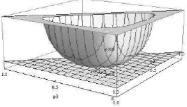
A three-dimensional numerical exampleWe consider the zero-order Markov process with final sequence of states X={x1, x2, x3, x1, x2, x3}. By
run-ning the programs from Section 6.1 and Section 6.2, we obtain
E(T(p)) =−1 + (p1p2p3)−1+ (p1p2p3)−2,
the optimal distribution p∗ = (1/3,1/3,1/3) and the optimal evolution timeE(T(p∗)) = 755.
The graph of the functionE(T(p)) of the variablesp2 andp3 is obtained by running the following instruction: P lot3D[{DG1, solF in[[2]]},{p2, eps,1−eps},
{p3, eps,1−p2−eps}, AxesOrigin→ {0,0,0}, AxesLabel→ {”p2”,”p3”,”E(T(p))”},
P lotRange→ {{0,1},{0,1},{0,5000}}]
[image:8.595.330.527.421.545.2]Figure 2. The graph of the three-dimensional example.
7
Conclusions
In this paper the following results were established:
• analysis of the zero-order Markov processes with fi-nal sequence of states and unit transition time;
• optimization of the existing algorithm for determi-ning the distribution of evolution time;
• optimization of the expectation of evolution time by applying geometric programming approach;
• implementation of the obtained methods by using Wolfram Mathematicar package;
• verification of the obtained scientific results by tes-ting the implemented versions for various numerical examples.
These results can be used in the theory of Markov pro-cesses and its applications.
Acknowledgements
This material is supported by 13.08.819.05F Inde-pendent Project for Young Researchers ”Numerical Me-thods for Solving Variational and Stochastic Optimal Control Problems”. The author thanks the scientific researchers who contributed with their suggestions and comments regarding this paper.
REFERENCES
[1] E. Andersen, Y. Ye. A computational study of the ho-mogeneous algorithm for large-scale convex optimiza-tion, Comput. Optim. Appl., No. 10(3), 243-269, 1998.
[2] M. Avriel, R. Dembo, U. Passy. Solution of generalized geometric programs, Int. J. Numer. Methods Eng., No. 9(1), 149-168, 1975.
[3] S. Boyd, S. Kim, L. Vandenberghe, A. Hassibi. A tu-torial on geometric programming, Optim. Eng., Educa-tional Section, Springer, No. 8, 67-127, 2007.
[4] S. Boyd, L. Vandenberghe. Convex optimization, Cam-bridge University Press, CamCam-bridge, 2004.
[5] R. Duffin. Linearizing geometric programs. SIAM Rev., No. 12(2), 668-675, 1970.
[6] R. Duffin, E. Peterson, C. Zener. Geometric programming-theory and application, Wiley, New York, 1967.
[7] R. A. Howard. Dynamic Probabilistic Systems, Wiley, 1972.
[8] R. A. Howard. Dynamic Programming and Markov Pro-cesses, Wiley, 1960.
[9] Q. Hu, W. Yue. Markov Decision Processes with Their Applications, Springer-Verlag, 2008.
[10] K. Kortanek, X. Xu, Y. Ye. An infeasible interior-point algorithm for solving primal and dual geometric pro-grams, Math. Program., No. 76(1), 155-181, 1996.
[11] A. Lazari. Algorithms for Determining the Transient and Differential Matrices in Finite Markov Processes, Bulletin of the Academy of Science of RM, No. 2(63), 84-99, 2010.
[12] A. Lazari. Compositions of stochastic systems with final sequence states and interdependent transitions, Annals of the University of Bucharest (mathematical series), Vol. LXII, No. 4, 289-303, 2013.
[13] A. Lazari. Evolution time of composed stochastic sys-tems with final sequence states and independent tran-sitions, Annals of the Alexandru Ioan Cuza University - Mathematics, Iasi, Romˆania, accepted.
[14] A. Lazari. Probabilistic characteristics of the evolution time of discrete random systems (in romanian), Studia Universitatis, CEP USM, No. 2(22), 5-16, 2009.
[15] A. Lazari. Numerical methods for solving deterministic and stochastic problems in dynamic decision systems (in romanian), PhD thesis in mathematics and physics, Chi¸sin˘au, 2011.
[16] D. Lozovanu, A. Lazari. An Approach for Determining the Matrix of Limiting State Probabilities in Discrete Markov Processes, Bulletin of the Academy of Science of RM, No. 1(62), 77-91, 2010.
[17] D. Lozovanu, S. Pickl. Algorithms for Determining the State-Time Probabilities and the Limit Matrix in Markov Chains, Bulletin of the Academy of Science of RM, No. 1(65), 66-82, 2011.
[18] Y. Nesterov, A. Nemirovsky. Interior-point polynomial methods in convex programming, Studies in applied mathematics, SIAM, Philadelphia, Vol. 13, 1994.
[19] E. Peterson. The origins of geometric programming, Ann. Oper. Res., No. 105(1-4), 15-19, 2001.
[20] M. Puterman. Markov Decision Processes, Wiley, 1993.
[21] J. Rajpogal, D. Bricker. Posynomial geometric gramming as a special case of semi-infinite linear pro-gramming, J. Optim. Theory Appl., No. 66(3), 444-475, 1990.
[22] W. J. Stewart. Probability, Markov Chains, Queues and Simulation, Princeton University Press, 2009.
[23] V. Ungureanu. Mathematical Programming. Chisinau, USM, 2001.
[24] D. Wilde, C. Beightler. Foundations of optimization. Prentice Hall, Englewood, Cliffs, 1967.