Multistable Perception in Schizophrenia: A
Model-based Analysis via Coarse-grained Order
Parameter Dynamics and a Comment on the 4th Law
T.D. Frank
Department of Psychology, Center for the Ecological Study of Perception and Action, University of Connecticut, 406 Babbidge Road, Storrs, 06269, Connecticut, United States
∗Corresponding Author: [email protected]
Copyright c⃝2014 Horizon Research Publishing All rights reserved.
Abstract
The synergetic computer that has originally been developed as an algorithm for pattern recognition has also been used in the life sciences as a model for various self-organizing perceptual processes. Coarse-graining of the order parameter equations of the synergetic computer is discussed for sets of to-be-perceived patterns that vary in the degree to which they can be distinguished from each other. Coarse-gaining is exploited to conduct a model-based analysis on literature data of multistable perception under schizophrenia as tested in motion-induced blindness (MIB) experiments. The analysis not only supports earlier sugges-tions that schizophrenia reduces the occurrence frequency of the MIB effect but also suggests that the perceptual system of schizophrenia patients is characterized by a greater degree of asymmetry.Keywords
Schizophrenia, Motion-induced Blindness, Self-organization, Order Parameter Dynamics, Dynamical Systems Modeling1
Introduction
The synergetic computer is an algorithm for pattern recog-nition [1]. The algorithm is based on self-organization prin-ciples and has been developed within the framework of syn-ergetics [2]. Although the algorithm has been developed to solve pattern recognition problems [1, 3, 4, 5, 6, 7], it has been generalized and applied in various related, interdisci-plinary fields. In particular, the algorithm has been gen-eralized to allow for hierarchical pattern recognition pro-cesses [8]. Economic and industrial applications in the field of settlement dynamics [9, 10], job assignment problems and robotics [11, 12, 13, 14, 15, 16, 17], and signal transmis-sions by means of a telecommunication (message) buffer [18] have been addressed. Although the synergetic com-puter describes an artifical associative memory or decision-making system, due to its roots in synergetics and the the-ory of self-organization, the synergetic computer has also been regarded as a benchmark model for self-organizing
psy-chological processes and self-organizing motor control sys-tem. In this context, oscillatory phenomenon induced by cer-tain perceptual [19, 20], and auditory [21, 22] stimuli have been discussed and application to priming [23, 24], grasp-ing [25, 26, 27], motor development durgrasp-ing infancy [28, 29], and bipolar disorder [30] can be found in the literature.
The pattern recognition algorithm is a winner-takes-all system that for a given initial stimulus pattern converges to a fixed point solution indicating the perception of a stored prototype pattern. The algorithm can be discussed from the perspective of the to-be-perceived and stored patterns. Al-ternatively, the algorithm can be studied from the perspec-tive of the pattern amplitudes. In line with the fact that the synergetic computer is considered as a computational or artificial organizing system mimicking natural self-organizing systems, the amplitudes have typically been con-sidered as order parameters [1, 31, 32].
Letξk denote the order parameters ofk = 1, . . . , N
pat-terns. We consider the order-parameter dynamics of the syn-ergetic computer in the following form [1]
d
dtξk =ξk
λ−B
N
∑
m̸=k,m=1
ξm2 −C
N
∑
m=1
ξm2
(1)
withλ, B, C >0. Equation (1) can be cast into a form that is convenient for conducting a stability analysis of fixed points in the generalized case that will be considered in Section 3 when the attention parameter λdepends on the pattern in-dex [7, 23, 24, 25, 26, 28]. Accordingly, (1) can equivalently be expressed by dξk/dt=ξk(λ−g C
∑N
m̸=k,m=1ξ 2
m−Cξk2),
where we have introduced the coupling parameterg = 1 +
B/C > 1. The parameterCcan be put toC = 1without loss of generality such that
d
dtξk =ξk
λ−g
N
∑
m̸=k,m=1
ξm2 −ξk2
. (2)
Alternatively, the parameter λand the order parameters ξk
parameters remain semi-positive definite for all times (i.e., ξk(t)>0∀t≥0).
In what follows, we will derive order parameter equations on several levels of coarse-graining. The ideas that will be developed below are closely related to the ideas developed in earlier studies on hierarchical generalizations of the order pa-rameter equations of the synergetic computer [8]. With these mathematical tools at hand, we will address multistable per-ception in schizophrenia. Finally, a comment on the clinical relevance of the 4th law of perceptual and behavioral transi-tions of living systems will be given.
2
Approximative coarse-grained
or-der parameter dynamics
In Section 2.1, we will consider first a special case that will be used in Section 3 in the application for multistable perception of schizophrenia. Subsequently, in Section 2.2, the general case will be discussed.
2.1
Special case
In this section, it is assumed that all patternsk= 2, . . . , N possess a common feature that is not present in the ’default’ patternk = 1. In this special case, we consider the course-grained order parameterU defined by
U =√ ∑
s∈IU
ξ2
s (3)
with the index set IU = {2, . . . , N}. Due to the
’winner-takes-all’ property of the synergetic computer (see Section 1) it follows that if one of the order parametersξk∗withk∗∈IU
becomes finite in the stationary case, thenU =ξk∗ >0. If
the order parameterξ1 of the default pattern becomes finite
in the stationary case, thenU = 0.
Before exploiting the definition (3), it is useful to cast the order parameter equations (2) of the synergetic computer in yet another form. (2) can be written like
d
dtξk=ξk
(
λ−g
N
∑
m=1
ξm2 −(1−g)ξk2
)
, (4)
where the mixed term contains the sum of all squared or-der parameters. Note that in (4) the cubic term ξ3
k
actu-ally has a positive coefficient because ofg > 1 (or since
−(1−g) =B >0holds usingC = 1again). Substituting the definition (3) into (4), we obtain
d
dtξ1 = ξ1
(
λ−g[U+ξ21]−(1−g)ξ12) , d
dtU = U
(
λ−g[U+ξ12]
)
−(1−g)1
U
∑
s∈IU
ξ4s.(5)
In the stationary case, we have either U = ξk∗ > 0 and
ξj̸=k∗ = 0if a patternk∗∈IUis selected orU = 0,ξk∈IU = 0,ξ1>0. In both cases, the dynamical system (5) forξ1and
U exhibits the same stationary fixed points as the coupled dynamical system
d
dtξ1,a = ξ1,a
(
λ−g[Ua+ξ12,a]−(1−g)ξ21,a
)
,
d
dtUa = Ua
(
λ−g[Ua+ξ12,a]−(1−g)U
2
a
)
(6)
for the variablesξ1,aandUa. Note that (6) assumes the form
of the order parameter equations of the synergetic computer again. The question arises to what extent the variablesξ1,a
andUacan be regarded as useful approximations to the order
parameterξ1and the coarse-grained order parameterU.
In this context, we first note that the expressionU4reads
U4=
[ ∑
s∈IU
ξs2
]2
= ∑
s∈IU
ξs4+mixed terms of the form(ξ2iξj2̸=i)
i,j∈IU .
(7) Consequently, (5) reads
d
dtξ1 = ξ1
(
λ−g[U+ξ12]−(1−g)ξ12) , d
dtU = U
(
λ−g[U+ξ12]−(1−g)U2)
+mixed 3rd order terms of the form 1
U
(
ξi2ξj2̸=i)i,j
∈IU . (8)
As indicated the mixed terms are considered third order terms because the products of order 4 are divided with the variable U that depends linearly on the scales of the variablesξk∈IU.
The dynamical systems (6) and (8) differ by the mixed terms occurring in theU-dynamics of the model (8). In or-der to assess the relevance of these terms, we apply a concept from psychophysics: the ’just noticeable difference’ (JND) of sensations [33]. We assume that all patterns under consid-eration differ from each other by a distance measureDthat will not be specified in detailed. For a human observer the patterns under consideration differ such that they can be dis-tinguished from each other. In this sense, for all pairs of pat-terns the distance measureDis larger than a certain threshold that corresponds to the JND.
Mathematically speaking, we assume that the initial condi-tions are such that the order parametersξk differ att= 0by
a certain amount that reflects the distanceDbetween the pat-terns and accounts for the aforementioned requirement that the sensation patterns (stimuli) under consideration differ at least by the JND. We distinguish between two cases.
Case I: It is assumed that patterns with a JND induce rel-ative large differences between the initial valuesξk(0)of the
order parameters. Accordingly, we assume that
∃k∗ : ∀j̸=k∗ : ξk∗(0)≫ξj(0). (9)
In this case, the order parameterξk∗ of the patternk∗will not
only win the selection process defined by (4) but the mixed terms in theU-dynamics of (8) will be negligibly small at all times relative to theU3term:
∀t≥0 : U3(t)≫mixed 3rd order terms of the form 1
U(t)
(
ξi2(t)ξj2̸=i(t))i,j
∈IU . (10)
If (10) holds, then the dynamical systems (6) and (8) ex-hibit approximately the same transient and stationary solu-tions. Consequently, the model (6) involving the variableUa
is a good approximative model for the original order param-eter model (4) of the synergetic computer. In particular, in the limiting caseξj̸=k∗(0)/ξk∗(0)→0a point-wise
Case I
A
ξ1
,
ξ1,a
[a
.u
.]
U
,U
a
[a
.u
.]
B
Time [a.u.]
Case II
C
Time [a.u.]
D
Case III
E
Time [a.u.]
[image:3.595.124.486.56.288.2]F
Figure 1. Illustrations of solutions for case I (A,B), II (C,D), III (E,F) initial conditions. Solutions of (4) (solid lines) and (6) (circles) are shown under consistent initial condition:ξ1,a(0) =ξ1(0),Ua(0) =U(0). See text for details. Parameters:N = 10,λ= 2.0,g = 1.3. Case I initial conditions:
ξ5(0) = 0.2,ξj̸=5(0) = 0.2/
√
(N−1)/10/(1 + 0.1ϵ). Case II:ξ5(0) = 0.2,ξj̸=5(0) = 0.2/
√
(N−1)/(1 + 0.2ϵ). Case III:ξ1(0) = 0.25,
ξj̸=1(0) = 0.2 + 0.01ϵ. In all cases,ϵwas uniformly distributed in[0,1].
pointtprovided that we use the consistent initial conditions ξ1,a(0) =ξ1(0)andUa(0) =U(0). An illustration is shown
in Fig. 1AB.
Case II: It is assumed that patterns with a JND induce dif-ferences between order parametersξk(0) that are scaled to
the size of the set of patterns and are at least of the magni-tude√N−1. More precisely, we assume that
∃k∗ : ∀j ̸=k∗ : ξk∗(0)> ξj(0)
√
N−1. (11) Let us distinguish between the two sub-cases thatk∗ ∈ IU
andk∗ ̸∈ IU (i.e.,k∗ = 1). Ifk∗ ∈ IU then the original
order parameter dynamics will converge to a fixed point with ξk∗ > 0 such that in the stationary caseU(st) = ξk∗(st)
holds. Moreover, it follows thatU(0) > ξk∗(0) > ξ1(0).
Consequently, if the dynamical system (6) is considered un-der consistent initial conditions (i.e., ξ1,a(0) = ξ1(0) and
Ua(0) = U(0)), thenUa converges to the finite stationary
valueUa(st) = U(st) = ξk∗(st) > 0 of the original
dy-namical system (4) andx1,a(t)converges to zero consistent
with the stationary behavior ofξ1: ξ1,a(st) = ξ1(st) = 0.
In contrast, if k∗ = 1then the original selection equation dynamics (4) converges to the fixed point withξ1 > 0and
U = 0. In addition, it follows that U2(0) = ∑
s∈IU
ξs2(0)< ∑
s∈IU
ξ2 1(0)
N−1 =ξ 2 1(0)
⇒U(0)< ξ1(0). (12)
If, again, the dynamical system (6) is considered under con-sistent initial conditions (i.e.,ξ1,a(0) = ξ1(0)andUa(0) =
U(0)), thenUa converges to the stationary valueUa(st) =
U(st) = 0andx1,a(t)converges to its finite fixed point value
consistent with the stationary behavior of ξ1: ξ1,a(st) =
ξ1(st) > 0. In summary, if condition (11) is satisfied, then
the dynamical system (6) involving the variableUa exhibits
the same stationary behavior than the original selection equa-tion model (4) provided that both dynamical systems are
con-sidered under consistent initial conditions. Figure 1CD ex-emplifies solutions of the dynamical systems (4) and (6) for this case.
In view of the fact that in the two aforementioned cases the performance of the dynamical model (6) is consistent in the stationary case with the original order parameter equation model (4) and given that both models exhibit formally the same mathematical structure, we will consider in what fol-lows the coupled differential equations (6) involving the vari-ablesξ1,a andUa as the (approximative) coarse-grained
or-der parameter equation model of the original synergetic com-puter model (4) (or (1)) involving the variablesξ1, . . . , ξN.
Finally, let us consider the general case in which neither of the two conditions described above are satisfied.
Case III: If the conditions considered in cases I and II are not satisfied, then the dynamical model (6) may exhibit so-lutions that are inconsistent with the order parameter dynam-ics (4) even if both dynamical models are solved under con-sistent initial conditions. Let us prove this statement by an ex-ample. Letξ1(0) =b >0andξk∈IU(0) =a >0withb > a.
For these initial conditions the original pattern recognition al-gorithm (4) converges to a fixed point withξ1(st) >0 and
ξk= 0fork∈IU indicating that the default patternk= 1is
recognized. Next, we consider the special case in which the distanceDbetween the default patternk = 1and the other patternsk≥2is not that large such that if the default pattern is presented we have b > abutb2 < (N −1)a2. That is,
the condition of case II is violated. Fromb2 < (N −1)a2
it follows thatU(0)2 = (N−1)a2> a2 =ξ2
1(0). In other
words, although forb > aandb2<(N−1)a2the condition ξ1(0)> ξk(0)holds for anyk ̸= 1, we haveU(0)> ξ1(0).
Consequently, if we solve the coarse-grained selection equa-tions (6) under consistent initial condiequa-tions (ξ1,a(0) =ξ1(0)
andUa(0) =U(0)), thenUa(t)converges to a finite
station-ary value Ua(st) > 0andξ1,a(t)converges to zero in the
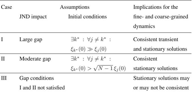
Table 1.Assumptions and implications for the correspondence of the fine- and coarse-grained amplitude dynamics
Case Assumptions Implications for the
JND impact Initial conditions fine- and coarse-grained dynamics
I Large gap ∃k∗ : ∀j̸=k∗ : Consistent transient ξk∗(0)≫ξj(0) and stationary solutions
II Moderate gap ∃k∗ : ∀j̸=k∗ : Consistent ξk∗(0)>
√
N−1ξj(0) stationary solutions
III Gap conditions Stationary solutions may
I and II not satisfied or may not be consistent
the original selection equations (4). Figure 1EF illustrates this case.
In summary, we have considered the special case in which the set ofN patterns under considerations exhibits a distinct default pattern andN −1patterns that constitute a class of non-default patterns. On a coarse-grained level, we consid-ered the order parametersξ1andU that describe whether a
pattern is recognized as the default pattern (ξ1(st) > 0)or as a pattern belonging to the class of non-default patterns (U(st) > 0). It was shown that for this special case a dy-namical model for the variablesξ1,aandUa can be derived
(see (6)) that under certain circumstances behaves approxi-matively in the same way asξ1 andU, respectively. More
precisely, if patterns are considered that differ at least by a JND that induces (i) a relative large gap or (ii) at least a gap of√N−1in the spectrum of initial amplitudesξk(0), then
in the stationary case the coarse-grained order parameter dy-namics involvingξ1,a andUa yields consistent results with
the fine-grained dynamics ofξ1, . . . , ξN. This implies that
the pattern selection made by the two dynamical systems is consistent. Under the condition (i) the two dynamical mod-els exhibit also approximatively the same transient solutions. If neither of the two gap conditions (i) and (ii) are satisfied, then the two models may yield inconsistent results. These considerations are summarized schematically in Table 1.
Importantly, the two dynamical models for the approxima-tive coarse-grained order parametersξ1,aandUaand for the
fine-grained order parametersξ1, . . . , ξNexhibit formally the
same mathematical structure.
Let us briefly address the assumptions listed in Table 1. The existence of a JND that induces the three gap condi-tions listed in Table 1 (labeled cases I, II, and III) depends on the circumstances under which perception is tested. From an evolutionary point of view it might be beneficial for the perceptional system to evolve in such a way that patterns fea-turing a JND induce the Case I condition. That is, a percep-tual system that is organized in the same way on different levels features a simpler or more parsimony architecture than a perceptual system that exhibits different organizations on different levels. Species endowed with this simpler architec-ture of their perceptual systems might have an evolutionary benefit over other species.
2.2
General case
Let us consider M levels of coarse-graining L ∈
{1, .., M}. The first level (L= 1) containsN1patterns. To
each pattern an order parameterξk,1is assigned that is used
to indicate whether the pattern is recognized. On the sec-ond level, patterns are grouped together such that there are N2 < N1 pattern classes. To each pattern class a
coarse-grained order parameterξk,2 is assigned that is used to
in-dicate whether a pattern out of the class is recognized. In general, each level exhibitsNL pattern classes (withN1 >
N2 >· · · > NM) that are described byNL coarse-grained
order parametersξk,L. For the sake of simplicity, the patterns
of levelL= 1and the corresponding amplitudesξk,1will be
treated as if they were pattern classes and pattern class am-plitudes, respectively.
At this stage, it is useful to introduce the index sets Ik,w=L+1 ⊂ {1, . . . , NL}. The index set Ik,w=L+1
con-tains all the pattern class indicesj from the coarse-grained levelLthat are grouped together to the classkof the coarse-grained levelL+ 1. For example, the index setIU discussed
in Section 2.1 we haveL = 1 ⇒ w = 2andIk=2,w=2 =
{2, . . . , N}. In general, the index sets Ik,w=L+1 satisfy
∀k ̸= j , k, j ∈ {1, . . . , NL+1} : Ik,L+1 ∩Ij,L+1 = ∅
and∪NL+1
k=1 Ik,L+1 = {1, . . . , NL}. In words, all index sets
belonging to a particular level of coarse-graining are mutu-ally disjunct and the unification of all index setsIk,w=L+1
gives the index set of all pattern classes of the coarse-grained level L. In analogy to (3), coarse-grained order parameters ξk,L+1are defined iteratively by
ξk,L+1=
√ ∑
s∈Ik,L+1
ξs,L2 . (13)
Let us assume that for a particular levelLof coarse-graining the selection equations forξk,Lassume the form of the order
parameter equations of the synergetic computer. In analogy to (4), we consider the selection equations
d
dtξk,L=ξk,L
(
λ−g
NL
∑
m=1
ξm,L2 −(1−g)ξk,L2
)
(14)
fork ∈ {1, . . . , NL}. Proceeding as in Section 2.1, we we
Appendix) d
dtξk,L+1= ξk,L+1
λ−g
N∑L+1
m=1
ξ2m,L+1−(1−g)ξ2k,L+1
(15) The selection equations (15) just assume the form of the order parameter equations of the previous levelL, see (14).
Finally, we assume that the patterns under consideration exhibit a JND that induces gap conditions as discussed in cases I and II of Section 2.1 for the initial amplitudesξk,L(0)
on all coarse-grained levelsL. Under these conditions, the mixed third order terms in (32) can be neglected (Case I) or affect the transient dynamics only to a relatively small de-gree (Case II). This implies that in both cases (Case I and II) the approximate selection equations (15) of the levelL+ 1
yield consistent results with the selection equations (14) of the levelL.
The assumptions made in the general case are the same as in Section 2.1 and consequently might be motivated in the same way. In addition, interestingly, we have formulated above the assumption that patterns of a levelLare uniquely mapped to pattern classes on the next levelL+ 1. That is, there is no pattern that belongs to two or more than two pat-tern classes. The assumption holds in the experiment that will be discussed in Section 3. However, it might be violated in other situations. Future work may be devoted to consider the case when a pattern can be member of several different pattern classes.
Let us exemplify the relationship between the selection equations (14) and (15) on subsequent levelsLandL+ 1
of coarse-graining. For illustration purposes it is sufficient to consider just two levelsM = 2and a set ofN1= 4patterns
onL = 1that is reduced toN2 = 2pattern classes on the
levelL= 2. Furthermore, the patternsk= 1,2andk= 3,4
onL= 1are assumed to constitute the pattern classesk= 1
andk = 2onL = 2. That is, we haveI1,2 = {1,2}and
I2,2 ={3,4}. ForL= 1the order parameter equations for
ξk,1withk= 1,2,3,4read
d
dtξk,1=ξk,1
(
λ−g
NL
∑
m=1
ξm,L2 −(1−g)ξ2k,1
)
(16)
and the coarse-grained order parameters on the levelL = 2
are defined by ξ1,2=
√
ξ2
1,1+ξ22,1, ξ2,2=
√
ξ2
3,1+ξ42,1. (17)
Under Case I and II initial conditions, the coarse-grained or-der parameters on levelL= 2satisfy at least approximately the selection equations
d
dtξ1,2=ξ1,2
(
λ−g[ξ12,2+ξ22,2]−(1−g)ξ12,2) , d
dtξ2,2=ξ2,2
(
λ−g[ξ21,2+ξ22,2]−(1−g)ξ22,2) . (18) Under case I initial conditions ∃k∗ : ξk∗,1(0) ≫
ξj̸=k∗,1(0) the solutions of the coarse-grained differential
equations (18) are good approximations to the exact solu-tions calculated from (16) and (17) provided consistent ini-tial conditionsξ2,1(0) =
√
ξ2
1,1(0) +ξ22,1(0)andξ2,2(0) =
ξ2
3,1(0) +ξ42,1(0)are used. In order to illustrate this
cor-respondence, we solved (16), (17), and (18) numerically, see Figure 2.
3
Motion-induced
blindness
and
schizophrenia
Motion-induced blindness is an optical illusion produced by a visual stimulus composed of a fixed stationary fore-ground pattern and a rotating backfore-ground pattern. Typically, the foreground pattern consists of three yellow dots arranged in a triangle, whereas the background pattern is a rotating ar-ray (or grid) of blue dots. A human observer exposed to the MIB stimulus typically reports that some of the target dots disappear for a while. In this sense, the motion of the back-ground pattern induces a temporary blindness with respect to the target pattern [34].
3.1
Modeling of fine- and coarse-grained
or-der parameter dynamics
We distinguish between 8 spatio-temporal patterns on the level L = 1that fall into two classes on the coarse-grained levelL= 2. There is one perceptual pattern not subjected to a MIB effect (i.e., the three yellow target dots are perceived), which is regarded as the default pattern indexed by k = 1
onL = 1. The default pattern constitutes its own class on L = 2Moreover, there are 7 different patterns that are sub-jected to a MIB effect (i.e., at least one dot is perceived as being absent). They are indexed byk = 2, . . . ,8onL= 1. and constitute the class of ’incomplete patterns’ on L = 2. On L = 2 the default pattern is index by k = 1 and the class of incomplete patterns is index byk = 2. Following earlier work on selective attention phenomena [1, 4], certain oscillatory phenomena of the perceptual [19, 20] and audi-tory system [21, 22], priming [23, 24], grasping [25, 26, 27], and child development [28, 29], we assume that in general the attention parameters of the two classes are different from each other. In this case, the evolution equations forL = 1
andL= 2read d
dtξk,1=ξk,1
λk,1−g
N
∑
m=1,m̸=k
ξm,2 1−ξk,21
(19)
fork= 1, . . . ,8and d
dtξ1,2 = ξ1,2
(
λ1,2−g U2−ξ21,2
)
,
d
dtU = U
(
λU−g ξ21,2−U2
)
(20) with λ1,1 = λ1,2 andλk,2 = λU for k = 2, . . . ,8. The
coarse-grained order parameter variables ξ1,2andU are
re-lated to the fine-grained order parameters ξ1,1, . . . , ξ8,1 as
discussed in the Section 2 with ξ1,2 ↔ ξ1,1 and U ↔
√∑8
k=2ξ2k,1.
The stability of the winner-takes-all fixed pointsξk∗,1 =
√
λk∗,1 ∧ ξj̸=k∗,1= 0of (19) and (ξ1,2=
√
λ1,2, U = 0),
(ξ1,2 = 0 , U =
√
λU) for (20) depend on the attention
ξ
3,1
,
ξ
2,2
[a
.u
.]
Time [a.u.]
A
U
,
ξ
1,2
[a
.u
.]
Time [a.u.]
[image:6.595.108.472.52.218.2]B
Figure 2.ξ1,2(panel A) andξ2,2(panel B) computed from (16) and (17) (solid lines) and (18) (circles) for consistent Case II conditions withξ3,1(0) = 0.2,
ξj̸=3(0) = 0.2/
√
(N−1)/(1 + 0.2ϵ),ϵuniformly distributed in[0,1], andN= 4,λ= 2,g= 1.3.
parameter spectrum has been discussed in detail in a series of studies [7, 23, 24, 25, 26, 28]. From these studies it follows that for the default pattern the stability depends onλ1,2,λU,
andglike
ξ1,1=
√
λ1,2 ∧ ξk≥2,1= 0
ξ1,2=
√
λ1,2 ∧ U = 0
}
=
{
stable if λ1,2> λU/g
unstable if λ1,2< λU/g
. (21) By analogy, for the incomplete patterns we have
∃k∗≥2 : ξk∗,1=
√
λU ∧ ξj̸=k∗,1= 0
ξ1,2= 0 ∧ U =
√
λU
}
=
{
stable if λU > λ1,2/g
unstable if λU < λ1,2/g
. (22) In what follows, we will primarily focus on the coarse-grained model. The oscillatory switching between the de-fault pattern and a pattern out of the class of incomplete pat-terns can be modeled by assuming that the attention param-etersλ1,2 andλU vary in time [18, 19, 20, 21, 22, 27, 30].
More precisely, we assume that if the default pattern is perceived thenλ1,2 decays gradually until the critical ratio
λ1,2 = λU/g is reached at which the percept becomes
un-stable, see (21). Consequently, the perceptual dynamics is subjected to a bifurcation and the perceptual experience of the default pattern is replaced by the percept of one of the in-complete patterns. However, the percept is assumed to induce again a decay in the corresponding attention parameter. That is,λUis assumed to decay gradually, whileλ1,2relaxes back
to a ’rest level of attention’. Among various possible dynam-ical systems that are able to capture these mechanisms, we will use the following evolution equations for the attention parameter dynamics:
d
dtλ1,2=−
1
τ(λ1,2(t)−b1,2), d
dtλU =−
1
τ(λU(t)−bU) (23) with
b1,2= 0 ∧ bU =b0 if ξ1,2=
√
λ1,2 ∧ U = 0
b1,2=b0 ∧ bU = 0 if ξ1,2= 0 ∧ U =
√
λU ,
(24)
whereb0denotes the aforementioned rest level andτ >0is
a time constant.
Our aim is to investigate the oscillatory dynamics (20), (23), (24) in a special case which allows for a semi-analytical approach. To this end, we note that the parameterτ defines the characteristic time scale of the attention parameter dy-namics. Likewise,1/λ1,2and1/λU define the characteristic
time scale of the dynamics of ξ1,2 andU. Let λc,low and
λc,high withλc,low > λc,high = gλc,low denote the
criti-cal attention parameters at which percept-switching occurs. Then λ1,2 and λU oscillate between these levels.
Conse-quently,ξ1,2(t)andU(t)evolve on a time scale at least as
fast as given by 1/λc,low. Ifλc,low is chosen large enough
(the value ofλc,lowdepends on the model parametersb0and
g) such that1/λc,lowis much shorter thanτ, then theξ1,2(t)
[image:6.595.305.537.592.645.2]andU(t)are fast evolve variables, whereas the attention pa-rameters λ1,2(t) and λU(t) are slowly evolving variables.
Figure 3 illustrates this case. In this case, the oscillation pe-riod can be calculated from the attention parameter dynamics alone. Moreover, differences in the transient behavior of the fine- and coarse-grained dynamics become irrelevant as long as both levels of consideration yield consistent results in the stationary case (case II, see Table 1).
In order to derive an expression for the oscillation period, we consider the case in whichλU decays from λc,high
to-wards zero andλ1,2relaxes back towardsb0:
λ1,2 = λc,lowexp
{
−t
τ
}
+b0
(
1−exp
{
−t
τ
})
,
λU = λc,highexp
{
−t
τ
}
. (25)
This phase will be terminated whenλ1,2=λc,highandλU =
λc,low. The duration of the phase corresponds to half of the
oscillation period. Therefore, att=T /2we have
λc,high = λc,lowexp
{
−T
2τ
}
+b0
(
1−exp
{
−T
2τ
})
,
λc,low = λc,highexp
{
−T
2τ
}
. (26)
Substituting λc,high = gλc,low into the second relation of
400 600 800 1000 1200
ξ
1,2
,
ξ
UTime [ms]
A
400 600 800 1000 1200
λ
1,
2
,
λ
UTime [ms]
[image:7.595.126.487.53.211.2]B
Figure 3.Oscillatory behavior of the order parameters (panel A)ξ1,2(solid),ξU(circles) and attention parameters (panel B)λ1,2(solid),λU(circles) for
τ= 100ms,g= exp{1},b0=g+ 1as computed from (20), (23), (24). Note that the observed period isT≈2τas expected.
Substitutingλc,high = gλc,low into the first relation of (26)
and taking (27) into account, we obtain a relationship be-tween the parametersb0andg:
b0=g+ 1. (28)
This relation tells us that the scenario described above can not be realized for any arbitrary values ofgandb0. Rather, the
model parameters must satisfy the matching condition (28). Eliminatingb0by means of (28), the model defined by (20),
(23), (24) involves two unknown parametersgandτ. If we fix one of the two parameters, then the remaining parameter can be estimated from the experimentally observed oscilla-tion periodTobs. In this context, a particular simple model
can be constructed if we putg =e(wheree= exp{1}). In this case, (27) reduces toT = 2τ, and the model parameter τcan be estimated from the observed oscillation periodTobs
likeτestim=Tobs/2.
Let us generalize the model in order to account for the fact that in MIB experiments the default percept and the in-complete percepts are not necessarily perceived for the same amount of time. That is, in general, the MIB paradigm in-volves perceptual oscillations composed of two phases with unequal durations. In order to introduce two phases with dif-ferent phase durations, we include a bias in the dynamical model defined by (20), (23), (24). To this end, (20) is re-placed by
dξ1,2
dt = ξ1,2
(
λ1,2+
δ
2 −g U 2−ξ2
1,2
)
,
dU
dt = U
(
λU −
δ
2 −g ξ 2 1,2−U2
)
. (29)
Forδ >0the duration of the phase withξ1,2>0andU= 0
becomes longer than the duration of the phase withξ1,2= 0
andU > 0. According to our interpretation of the model, we say that forδ > 0there is a bias towards perceiving the default pattern. Likewise, for δ < 0 the model reflects a perceptual systems exhibiting a bias towards the perception of an incomplete pattern. If we consider the parsimony model defined by (23), (24), and (29) with fixed parameters g = exp{1}andb0 =g+ 1, then we have two parametersτand
δat our disposal to model experimentally observed durations of the phase of default pattern perception and the phase of incomplete pattern perception.
3.2
Schizophrenia patients data versus
con-trols
Schizophrenia patients frequently show deficits in the per-ceptual processing of visual stimuli. In particular, perper-ceptual processes are affected that involve higher cognitive functions such as feature binding [35, 36, 37, 38]. On the other hand, there is evidence that the MIB phenomenon involves such higher cognitive processes and does not arise from low hi-erarchical processes like retinal suppression. For example, visual aftereffects that are assumed to emerge on a relative low hierarchical level of sensory processes are induced by the target dots of the MIB stimulus although these dots are not perceived by the observers [39, 40]. In other words, there is experimental evidence that when a target dot is not per-ceived by an observer then the sensory stimuli of the target dot is still processed in low hierarchical levels of the per-ceptual system but it is not processed (’correctly’) on higher cognitive levels involved in consciousness and sensory expe-riences that are explicit to the observer. This point of view is also supported by experimental studies that point out the similarity between the MIB phenomenon and other Gestalt theoretical phenomena such as perceptual filling-in [41]. In summary, higher cognitive functions are relevant both for the MIB phenomenon and our understanding of schizophrenia, which makes the MIB phenomenon a promising paradigm to investigate schizophrenia [42].
In a study by Tschacher et al. [42] controls and schizophre-nia patients were tested on the MIB phenomenon. Both groups were exposed to three trials of 60 seconds. On the av-erage, the number of total MIB experiences within these three minutes was about 42 for controls and 29 for patients (see Ta-ble 3 in [42]). In what follows we distinguish between total and single event durations. The total durations of the MIB ex-periences was about 42 seconds for controls and 33 seconds for patients. From these data we can obtain a crude measure for the duration of a single MIB event. For controls we obtain a single MIB duration of aboutTMIB= 1.0s (i.e., 42sec/42).
For patients we obtain a single MIB event duration dura-tion of about TMIB = 1.1s (i.e., 33sec/29). Likewise, we
Table 2.Descriptive experimental data and model parameters
Data Model
Group Tdefault[ms] TMIB[ms] τ[ms] δ[1/ms]
Controls 3300 1000 1500 1.6
Patients 4500 1100 1700 1.8
obtain an estimated single event duration ofTdefault = 3.3s
(i.e., 138sec/42). Likewise, for patients we obtain a single event duration of the default pattern of aboutTdefault = 4.5s
(i.e., 147sec/33). In view of (29), we anticipate that a model-based analysis of the data should reveal that the parameterδ is larger for schizophrenia patients because the asymmetry of the durations of the MIB and non-MIB phases is more pro-nounced.
We fitted the model parametersδandτ to reproduce the duration dataTMIBandTdefaultfor controls and patients. To
this end,τwas varied in the interval[Tdefault, TMIB]in steps
of 100 ms, whileδwas varied in the interval[0,2.0]1/ms in steps of 0.1. The results of this fitting procedure are summa-rized in Table 2. As expected, we found that the asymmetry parameterδis larger for schizophrenia patients than for con-trols.
4
Discussion
We studied coarse-graining of order parameter equations of the synergetic computer and followed in part earlier stud-ies on hierarchical generalizations of the synergetic com-puter concept [8]. In particular, we showed that under cer-tain conditions the coarse-grained order parameter equations exhibit the same mathematical structure as the correspond-ing fine-grained order parameter equations. In this sense, self-organizing artificial and natural systems, whose dynam-ics can be described (at least to some approximation) by the synergetic computer equations, exhibit a scale free system dynamics. A model-based analysis of literature data on mul-tistable perception of schizophrenia patients tested in an MIB experiment was carried out. The observation that the fre-quency of MIB experiences is lower for schizophrenia pa-tients than for controls corresponds in the model to a time scale parameter τ that is larger for schizophrenia patients than for controls. In addition, the model-based analysis high-lights a second perceptual characteristics of schizophrenia patients that has so far received only little attention. The two different perceptual phases in MIB experiments seem to be less symmetric in duration under schizophrenia. This shows up as a symmetry breaking parameterδ which is larger for schizophrenia patients than for controls.
We have shown that the model-based analysis of percep-tual data from schizophrenia patients and controls allow us to estimate model parameters that are difficult to measure directly. In addition, the model-based analysis may be ex-ploited to speculate about the clinical relevance of the so-called 4th law of systems that operate far from thermody-namic equilibrium. The 4th law claims that perceptual and behavioral transitions in living systems and in intelligent sys-tems in general occur in such a way that the rate of entropy
production is maximized [43, 44]. That is, the 4th law de-fines a selection principle. Interestingly, the stability condi-tions (21) and (22) define a similar maximization principle. Accordingly, when schizophrenia patients and controls expe-rience a change in the perception, this transition is accompa-nied with an increase from a relative low attention parameter to a relative high attention parameter. In other words, when the perceptual system undergoes a transition, then it selects a percept out of all possible percepts such that the magnitude of the attention parameter increases. This selection princi-ple does not only apply for the MIB model discussed above but holds in general for Haken’s amplitude equations of pat-tern formation systems [23, 24, 28]. Most importantly, it has been advocated that the two selection principles have a com-mon basis. For a large class of systems it has been shown that the attention parameters can be regarded as measures for the rate of entropy production [18, 45]. Consequently, for such systems and in particular for the perceptual-cognitive system tested under the MIB paradigm we are inclined to say that the 4th law applies and that transitions happen in such a way to increase the rate of entropy production. As mentioned above and as illustrated in Table 2, the symmetry breaking param-eterδreflecting the bias towards the perception of the com-plete pattern is larger for schizophrenia patients than for con-trols. This implies that the total attention (defined in terms of the attention parameter plus the parameterδ) towards the complete patterns is larger for schizophrenia patients than for controls. Likewise the total attention towards incomplete pat-terns is smaller for schizophrenia patients than for controls. In terms of entropy production this means that the rate of entropy production during perception of complete patterns is higher for schizophrenia patients than for controls. Vice versa the rate of entropy production during perception of in-complete patterns is lower for schizophrenia patients than for controls. In line with the argument (related to the 4th law) that living system favor perceptual and behavioral con-ditions that allow them to dissipate energy quickly (i.e., have to tendency to maximize the rate of entropy production), we may reverse the chain of the arguments and speculate that un-der schizophrenia the rate of entropy production is increased (relative to controls) if complete or whole patterns are per-ceived. Accordingly, higher rates of entropy production un-der schizophrenia during perception of complete patterns is the reason why in MIB experiment under schizophrenia the duration of MIB experiences (i.e., the duration of experiences of incompleteness) is shorter.
Appendix
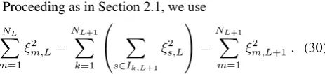
Proceeding as in Section 2.1, we use
NL
∑
m=1
ξm,L2 =
N∑L+1
k=1
∑
s∈Ik,L+1 ξ2s,L
=
N∑L+1
m=1
ξm,L2 +1. (30)
Differentiating (13) with respect to time t and substituting (14) and (30) into the resulting equation, we obtain in analogy to (5) the following result
d
dtξk,L+1 = ξk,L+1
λ−g
N∑L+1
m=1
ξm,L2 +1
−(1−g) 1
ξk,L+1
∑
s∈Ik,L+1
fork ∈ {1, . . . , NL+1}. Using the same line of arguments
as in Section 2.1, the most right standing term in (31) can be expressed in terms ofξk,L+1and mixed terms of the form
ξ2i,Lξj,L2 withi̸=j. Consequently, in analogy to (8), (31) can be cast into the form
d
dtξk,L+1= ξk,L+1
λ−g
N∑L+1
m=1
ξ2m,L+1−(1−g)ξ2k,L+1
+mixed 3rd order terms of the form 1
ξk,L+1
(
ξ2i,Lξj2̸=i,L)i,j
∈Ik,L+1 . (32) Neglecting the third order mixed terms, we obtain a coupled set of approximate selection equations of the coarse-grained levelL+ 1defined by (15), see main text.
Acknowledgments
TDF is very grateful to Dobromir Dotov for his help in preparing this study. Preparation of this manuscript was sup-ported in part by National Science Foundation under the IN-SPIRE track, grant BCS-SBE-1344275.
REFERENCES
[1] H. Haken, Synergetic computers and cognition, Springer, Berlin, 1991.
[2] H. Haken, Synergetics: Introduction and advanced topics, Springer, Berlin, 2004.
[3] H. Haken, Nonequilibrium phase transitions in pattern recog-nition and associative memory, Z. Physik B 70 (1988) 121– 123.
[4] A. Fuchs, H. Haken, Pattern recognition and associative mem-ory as dynamical processes in a synergetic system. I. Trans-lational invariance, selective attention and decomposition of scene, Biol. Cybern. 60 (1988) 17–22.
[5] A. Fuchs, H. Haken, Pattern recognition and associative mem-ory as dynamical processes in a synergetic system. II. Decom-position of complex scenes, simultaneous invariance with re-spect to translation, rotation, and scaling, Biol. Cybern. 60 (1988) 107–109.
[6] A. Daffertshofer, H. Haken, A new approach to recognition of deformed patterns, Pattern recognition 27 (1994) 1697–1705.
[7] T. D. Frank, New perspectives on pattern recognition algo-rithm based on Haken’s synergetic computer network, in: M. D. Fournier (Ed.), Perspective on pattern recognition, Nova Publ., New York, 2011, pp. Chap. 7 (pp. 153–172).
[8] A. Daffertshofer, H. Haken, Adaptive hierarchical structures, in: J. Mira, F. Sandoval (Eds.), From natural to artifical neu-ral computation. Lecture notes in computer science, Vol. 930, Springer, Berlin, 1995, pp. 76–84.
[9] A. Daffertshofer, H. Haken, J. Portugali, Self-organized set-tlements, Environ. Plann. B 28 (2001) 89–102.
[10] A. Daffertshofer, How do ensembles occupy space?, Eur. Phys. J. Special Topics 157 (2008) 79–91.
[11] J. Starke, M. Schanz, H. Haken, Treatment of combinato-rial optimization problems using selection equations with cost terms. Part II, Physica D 134 (1999) 242–252.
[12] J. Starke, T. Kaga, M. Schanz, T. Fukuda, Experimental study on self-organized and error resistant control of distributed autonomous robotic systems, Int. J. Robotics Research 24 (2005) 465–486.
[13] J. Starke, M. Schanz, Dynamical system approaches to combi-natorial optimization, in: D. Z. Du, P. Pardalos (Eds.), Hand-book of combinatorial optimization, Vol. 2, Kluwer Aca-demic Publisher, Dordrecht, 1998, pp. 471–524.
[14] J. Starke, C. Ellsaessar, T. Fukuda, Self-organized control in cooperative robots using a pattern formation principle, Phys. Lett. A 375 (2011) 2094–2098.
[15] H. Haken, Decision making and optimization in regional plan-ning, in: M. Beckmann, B. Hohannsson, F. Snickars, R. Thord (Eds.), Knowledge and networks in a dynamic economy, Springer, Berlin, 1998, pp. 25–40.
[16] H. Haken, M. Schanz, J. Starke, Treatment of combinato-rial optimization problems using selection equations with cost terms. Part I, Physica D 134 (1999) 227–241.
[17] T. D. Frank, Multistable selection equations of pattern forma-tion type in the case of inhomogeneous growth rates: with applications to two-dimensional assignment problems, Phys. Lett. A 375 (2011) 1465–1469.
[18] T. D. Frank, Rate of entropy production as a physical selec-tion principle for mode-mode transiselec-tions in non-equilibrium systems: with an application to a non-algorithmic dynamic message buffer, European Journal of Scientific Research 54 (2011) 59–74.
[19] T. Ditzinger, H. Haken, Oscillations in the perception of am-bigious patterns: a model based on synergetics, Biol. Cybern. 61 (1989) 279–287.
[20] T. Ditzinger, H. Haken, Impact of fluctuations on the recogni-tion of ambiguous patterns, Biol. Cybern. 63 (1990) 453–456.
[21] T. Ditzinger, B. Tuller, J. A. S. Kelso, Temporal patterning in an auditory illusion: the verbal transformation effect, Biol. Cybern. 77 (1997) 23–30.
[22] T. Ditzinger, B. Tuller, H. Haken, J. A. S. Kelso, A synergetic model for the verbal transformation effect, Biol. Cybern. 77 (1997) 31–40.
[23] T. D. Frank, On a multistable competitive network model in the case of an inhomogeneous growth rate spectrum with an application to priming, Phys. Lett. A 373 (2009) 4127–4133.
[24] T. D. Frank, Psycho-thermodynamics of priming, recogni-tion latencies, retrieval-induced forgetting, priming-induced recognition failures and psychopathological perception, in: N. Hsu, Z. Sch¨utt (Eds.), Psychology of priming, Nova Publ., New York, 2012, pp. Chap. 9 (pp. 175–204).
[25] T. D. Frank, M. J. Richardson, S. M. Lopresti-Goodman, M. T. Turvey, Order parameter dynamics of body-scaled hys-teresis and mode transitions in grasping behavior, J. Biol. Phys. 35 (2009) 127–147.
[27] S. M. Lopresti-Goodman, M. T. Turvey, T. D. Frank, Negative hysteresis in the behavioral dynamics of the affordance ”gras-pable”, Attention, Perception, and Psychophysics 75 (2013) 1075–1091.
[28] T. D. Frank, J. van der Kamp, G. J. P. Savelsbergh, On a mul-tistable dynamic model of behavioral and perceptual infant development, Dev. Psychobiol. 52 (2010) 352–371.
[29] T. D. Frank, Motor development during infancy: a nonlin-ear physics approach to emergence, multistability, and sim-ulation, in: A. M. Columbus (Ed.), Advances in psychology research, Vol. 83, Nova Publ., New York, 2011, pp. Chap. 9 (pp. 143–160).
[30] T. D. Frank, From systems biology to systems theory of bipo-lar disorder, in: F. Miranda (Ed.), Systems theory: perspec-tives, applications and developments, Nova Publ., New York, 2014, pp. Chap. 2 (pp. 17–36).
[31] M. Bestehorn, H. Haken, Associative memory of a dynamical system: an example of the convection instability, Z. Physik B 82 (1991) 305–308.
[32] T. D. Frank, Multistable pattern formation systems: can-didates for physical intelligence, Ecological Psychology 24 (2012) 220–240.
[33] J. B. J. Smeets, E. Brenner, Grasping Weber’s law, Current Biology 18 (2008) R1089–R1090.
[34] Y. S. Bonneh, A. Cooperman, D. Sagi, Motion-induced blind-ness in normal observers, Nature 411 (2001) 798–801.
[35] E. M. Rabinowicz, L. A. Opler, D. R. Owen, R. A. Knight, Dot enumeration perceptual organization task (DEPOT): evi-dence for a short-term visual memory deficit in schizophrenia, J. Abnormal Psychology 105 (1996) 336–348.
[36] P. J. Uhlhaas, S. M. Silverstein, The continuing relevance of Gestalt psychology for an understanding of schizophrenia,
Gestalt Theory: An International Multidisciplinary Journal 25 (2003) 256–279.
[37] P. J. Uhlhaas, S. M. Silverstein, Perceptual organization in schizophrenia spectrum disorders: empirical research and the-oretical implications, Psychological Bulletin 131 (2005) 618– 632.
[38] W. Tschacher, How specific is the Gestalt-informed approach to schizophrenia, Gestalt Theory: An International Multidis-ciplinary Journal 26 (2004) 335–344.
[39] C. Hofstoetter, C. Koch, D. C. Kiper, Motion-induced blind-ness does not affect the formation of negative afterimages, Consciousness and Cognition 13 (2004) 691–708.
[40] L. Montaser-Kouhsari, F. Moradi, A. Zandvakili, H. Es-teky, Orientation-selective adaptation during motion-induced blindness, Perception 33 (2004) 249–254.
[41] L. C. Hsu, S. L. Yeh, P. Kramer, Linking motion-induced blindness to perceptual filling-in, Vision Research 44 (2004) 2857–2866.
[42] W. Tschacher, D. Schuler, U. Junghan, Reduced perception of the motion-induced blindness illusion in schizophrenia, Schizophrenia Research 81 (2006) 261–267.
[43] R. Swenson, M. T. Turvey, Thermodynamic reasons for perception-action cycles, Ecol. Psychol. 3(4) (1991) 317–348.
[44] M. T. Turvey, C. Carello, On intelligence from first princi-ples: guidelines for the inquiry into the hypothesis of physical intelligence, Ecological Psychology 24 (2012) 3–32. [45] T. D. Frank, Pumping and entropy production in

![Figure 2.1√ξ ξ,2 (panel A) and ξ2,2 (panel B) computed from (16) and (17) (solid lines) and (18) (circles) for consistent Case II conditions with ξ3,1(0) = 0.2,̸j=3(0) = 0.2/(N − 1)/(1 + 0.2ϵ), ϵ uniformly distributed in [0, 1], and N = 4, λ = 2, g = 1.3.](https://thumb-us.123doks.com/thumbv2/123dok_us/8777955.902519/6.595.108.472.52.218/figure-computed-circles-consistent-case-conditions-uniformly-distributed.webp)